Chapter 8. Analyzing the Growth of Bitcoin Network Size with the Power Law and Square Root of Elapsed Time (SRET) Models
A 2018 change occurred in the growth rate of Bitcoin network size, demonstrated by both the Power Law and SRET models.
8.1 Overview
In Chapter 8, the application of the Power Law and the SRET models to the growth of Bitcoin network size will be explored. The application of the Power Law and SRET models to the growth of Bitcoin network value (i.e., market cap) will be the topic of Chapter 9.
In Chapters 6 and 7, modeling of technology adoption by the Power Law and SRET models was explored for 14 historic technology adoptions of the 20th and 21st centuries, including the recent/ongoing worldwide adoptions of internet access and cell phones.
The 7 technology adoptions in Chapter 6 were effectively modeled by both the Power Law model and the SRET model, although the Power Law model was somewhat more effective. These technology adoptions were marked by rapid growth with moderate annual growth deceleration.
The 7 technology adoptions in Chapter 7 were effectively modeled by the SRET model, but not by the Power Law model with 0 time adjustment.
Therefore, in Chapter 8, modeling the growth of Bitcoin network size follows a sequence outlined in Chapter 7.
Model network growth using the SRET approach. This “gentler” modeling approach identified appropriate adoption periods in each of the 14 previous technology adoptions of Chapters 6 and 7.
Model network growth using the Power Law with 0 time offset. Evidence that this model is not working includes:
Data in early adoption periods is convex rather than linear; and/or
Two early adoption periods are apparent when the SRET model demonstrated a single adoption period; and/or
Early adoption periods by the Power Law model don’t match the early adoption periods of the SRET model.
There is a discontinuity in the transition between adoption periods.
Examine the Power Law with positive offset values — to determine the value of the time offset that eliminates Power Law model discontinuities between adoption periods. The correct value of the time offset will lead to Power Law identification of the same adoption periods identified with the SRET model.
8.2. Market Cap and Bitcoin-Containing Addresses as Proxies for Network Value and Network Size
The task of modeling the growth of Bitcoin network size and network value begins with choice of suitable metrics. Bitcoin market capitalization is the logical metric for network value. Bitcoin-containing address count is the proposed metric for network size.
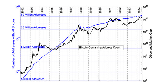
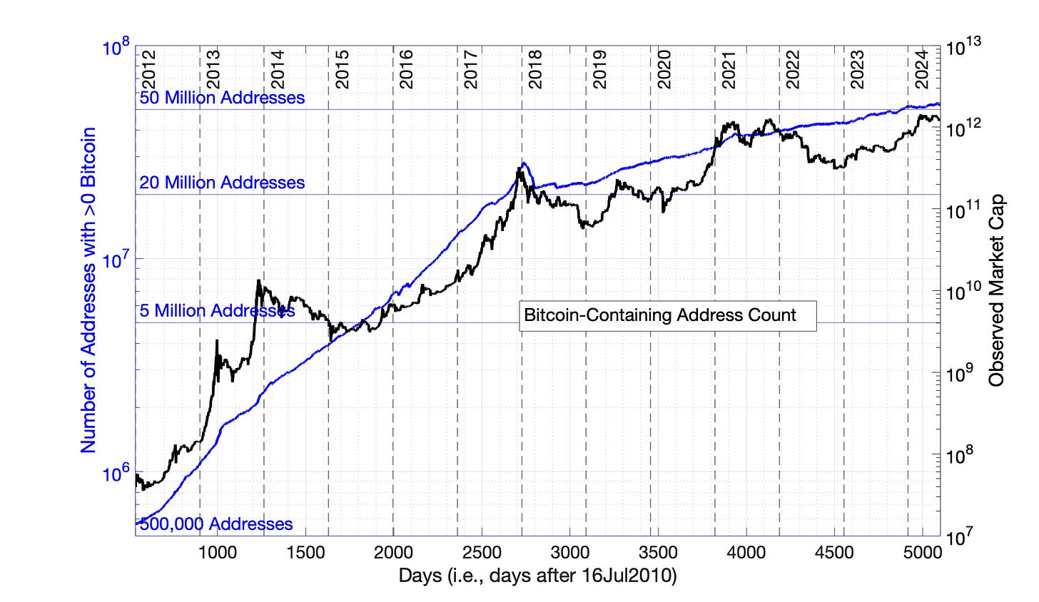
Daily values for market cap and Bitcoin-containing addresses are available starting 17Jul2010 — Day 1 of Bitcoin price history in the Glassnode database. Bitcoin-containing addresses stabilized as a representation of network size at the beginning of 2012. Bitcoin-containing addresses and market cap from 01Jan2012 to 01Jul2024 are presented as a semilog plot in Fig 8.1.
Fig 8.1 Semilog plots of the number of Bitcoin-containing addresses and Bitcoin market cap vs. elapsed time. Market capitalization in USD is plotted for (in black), with reference to the values on the right Y-axis. Day 1 is set as 17Jul2010, the first day of Bitcoin price history in the Glassnode database.
The strongest evidence for the suitability of Bitcoin-containing address count as a metric for the growth of Bitcoin network size comes from its success in confirming one of the most important early network value models. Robert Metcalfe proposed that for many networks, network value and network size should be related by the equation V = c*N2, where V is network value, N is network size, and c is a constant.
Metcalfe’s logic was as follows. For a network with 5 participants, A, B, C, D and E, the ten possible interactions are AB, AC, AD, AE, BC, BD, BE, CD, CE and DE. If P is the number of participants, the number of combinations is P*(P-1)/2 — so, 5 participants leads to 5*4/2 = 10 combinations. As P gets very large, the relationship P*(P-1) approaches P2 .
In such a network, Robert Metcalfe proposed relationship network value and network size as V = c*N2, where V = network value, N = network size, and c is a constant (Ref 1). He then demonstrated this concept with data from the growth of network value and network size for Facebook (Ref 1). Several previous publications have reported that the Bitcoin network followed this relationship between 2012 and 2018 (References 2 to 5).
The suitability of Bitcoin-containing address count as a suitable metric for Bitcoin network size comes from a demonstration that this metric satisfied Metcalfe’s Law in the period from 2012 to 2018.
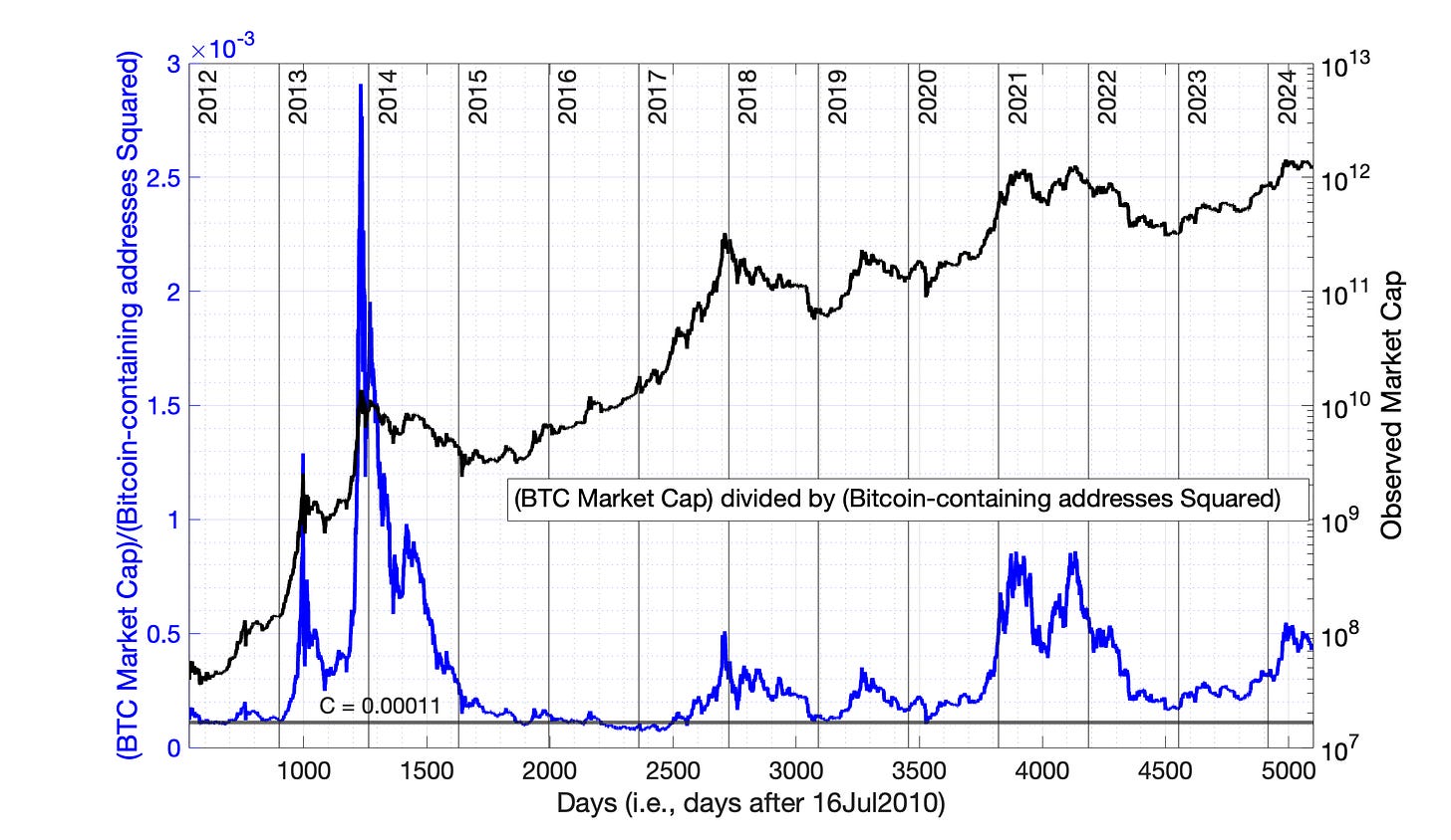
If V = c*N2, then V/N2 = c. The premise that Bitcoin-containing address count is a suitable metrics for Bitcoin network size is tested by plotting the ratio V/N2 as a function of time, where V and N are represented by Bitcoin market cap and Bitcoin-containing addresses, respectively Periods in which Metcalfe’s Law is followed will have constant V/N2 (See Fig 8.2).
Focussing on the period between 2012 and the end of 2018: In Figure 8.2, the ratio, c, is constant at approximately 0.00011 only during the periods before and after the 2013 and 2017 “bull runs.”
To put the relationship V = c*N2 in context, between July, 2012 and April, 2016, Bitcoin-containing address count grew from about 750,000 to 7,500,000, a 10-fold increase (Fig 8.1.) During that same period, the Bitcoin fair value market cap from Fig 8.1 grew from about $80 Million to $8 Billion, a 100-fold increase. A 10-fold increase in network size resulted in a 100-fold increase in network value, consistent with Metcalfe’s Law.
During the 2013 and 2017 “bull market” periods, network value ceased to be a function of network size. The value of V/N2 rose about 30-fold and 5-fold above baseline at the peaks of the 2013 and 2017 “bull markets.” (Fig 8.2) Yet after those “bull market” periods, the market value returned in each case to a baseline where V/N2 = 0.00011.
The baseline in Fig 8.2 appears to drift higher than 0.00011 after 2019. This is probably related to the regime change that occurred in the Bitcoin network after 2018/2019.
The data of Fig 8.2 support the premise to be carried forward in these Substack chapters that:
Bitcoin-containing addresses is a suitable candidate to represent Bitcoin network size. It is not necessary that this metric be an absolute measure of network size. Rather, it is only necessary that it is proportional to network size.
The historic Bitcoin “bull markets” of 2013, 2017, 2019, and 2021 were temporary price bubbles in which Bitcoin market cap detached from its relationship to Bitcoin network size. The models to be developed in these Substack chapters will focus on the periods between these Bitcoin price bubble episodes, the “non-bubble periods” of Bitcoin history.
Fig 8.2 The Bitcoin network follows Metcalfe’s Law in the periods between 2012 and 2018, but only during the periods between “bull runs.” The ratio V/N2 is plotted from 01Jan2012 to 01Jul2024, where market cap and Bitcoin-containing addresses are the metrics for V and N, respectively. This ratio is constant at a value of approximately 0.00011 in the periods before and after the “bull runs” of 2013 and 2017, with some baseline oscillation due to Bitcoin price volatility. Observed market capitalization in USD is plotted for comparison (in black), with reference to the right Y-axis.
8.3 Modeling Bitcoin-Containing Address Count with the SRET Model
The Bitcoin-containing address metric became a stable measure of network size starting in about January, 2012. Therefore, this is typically the starting point for modeling in these Substack chapters is 01Jan2012, Day 534.
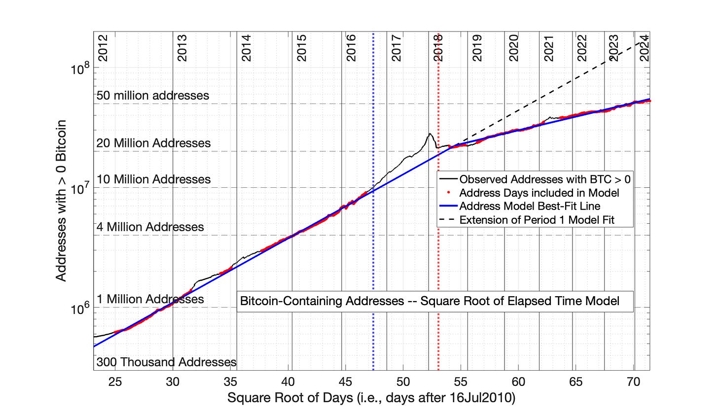
Bitcoin-containing addresses is plotted in the SRET model format in Fig 8.3. The data is modeled in two periods: Period 1, from 01Jan2012 to 01Sep2018 and Period 2, from 01Sep2018 to 01Jul2024. The date 01Sep2018 was identified by trial and error as the approximate transition point between Periods 1 and 2.
The Square Root of Elapsed Time (SRET) model equations for Period 1 and Period 2 in Figure 8.3 were developed as follows.
The model formula for a straight line in Period 1 or Period 2 is
ln(address count) = m*(square root of elapsed time) + b, where m and b are constants, the slope and intercept, respectively.
Identify a first guess for m and b. This can be accomplished by algebraically determining starting values of m and b from two points along a hand-drawn line through the relevant data.
Then, identify the subset of “red” data points plus-or-minus 5% of that straight line, and compute a least-squares, best-fitting, straight line through these “red”, data points. This invariably identifies a new line — a new m and b. (The range of plus-or-minus 5% was determined to ignore address data associated with Bitcoin price bubbles, during which the Bitcoin-containing address count grew temporarily above trend.)
Identify a new subset of “red”,data points plus-or-minus 5% of that new straight line, then compute a new least-squares, best-fitting, straight line through these “red” data points, a new m and b.
Repeat this sequence until the algorithm convergences on a non-varying set of “red” fair-value data points, and a non-varying, least-squares best-fitting straight line, a final m and b.
This sequence has been repeated more than 100 times over the past 2 years in modeling Bitcoin addresses and Bitcoin market cap, by both the SRET and Power Law models. This sequence has always converged on a final solution for the m and b, provided that the initial guess of m and b is a realistic.
The results of this iterative process are presented in Fig 8.3 for Periods 1 and 2. The “red” fair-value data points in Period 1 represent 1264 of the 2435 total days in that period, while the “red” fair-value data points in Period 2 represent 1842 of the total 2130 days in that period. The data excluded from calculations are indicated in black. The excluded data include elevated address counts in the periods of the 2013, 2017 and 2021 price bubbles, and depressed address counts in a period following the price crash after the 2017 price bubble.
The final SRET model equations for the Period 1 and 2 “blue” lines in Fig 8.3 are:
Period 1: ln(Addresses) = 0.1230*(sqrt of elapsed time) + 10.22
Period 2: ln(Addresses) = 0.05262*(sqrt of elapsed time) + 14.06
The SRET model results of Fig 8.3 are plotted semilog as a function of time in Fig 8.4.
Fig 8.3 Bitcoin-containing addresses: the Square Root of Elapsed Time (SRET) model. Bitcoin-containing addresses are evaluated by the SRET model in 2 periods: Period 1: from 01Jan2012 to 01Sep2018 and Period 2: from 01Sep2018 to 01Jul2024. The least-squares, best-fitting straight lines are shown in solid blue for the two periods. These lines were based on the data points marked in red, which are within plus-or-minus 5% of the blue lines. A dashed, black line is the Period 1 relationship extrapolated into Period 2 — to help visualize the slope change occurring between Periods 1 and 2. The vertical, dotted red line represents the temporal midpoint of data presented on the x-axis, while the vertical, dotted blue line represents the visual midpoint of the x-axis data. Year designations (for January 1) are presented inside the graph at the top, and the corresponding Day number is presented inside the graph at the bottom. The R2 for Periods 1 and 2 were 0.999 and 0.993, respectively.
Fig 8.4. Bitcoin-containing addresses: SRET model results from Fig 8.3 plotted semilog versus time. The data and SRET model equations demonstrate the rapid, but decaying growth rate typical of technology adoptions. The meanings of the solid blue lines and the dashed black line are the same as Fig 8.3. In this semilog plot versus time, the dotted red and blue lines collapse into the same line — the temporal and visual midpoints of the graph are identical.
8.4 Modeling Bitcoin-Containing Address Count with the Power Law Model
Bitcoin-containing addresses were assessed with the Power Law model following the same procedure employed for the SRET model.
Separately model the data as two periods before and after 01Sep2018
Employ the same iterative procedure of Section 8.3 to determine the best-fitting slope and intercept for the model equations.
The results are presented as Figures 8.5, 8.7, and 8.9 for Power Law time offsets of 0 days, 560 days and 2000 days — for comparison to the SRET model results in Fig 8.3. In Figures 8.6, 8.8, and 8.10, the Power Law model results are plotted semilog as a function of time, for comparison to the SRET model results in Fig 8.4.
The model formulas for these four Power Law cases are
0-day offset (Fig 8.5):
Period 1. ln(Addresses) = 2.145*ln(elapsed time) - 0.6628
Period 2. ln(Addresses) = 1.687*ln(elapsed time) + 3.402
560-day offset (Fig 8.7):
Period 1. ln(Addresses) = 3.167*ln(elapsed time + 560) - 9.159
Period 2. ln(Addresses) = 1.905*ln(elapsed time + 560) + 1.345
2000-day offset (Fig 8.9):
Period 1. ln(Addresses) = 5.725*ln(elapsed time+ 2000) - 31.75
Period 2. ln(Addresses) = 2.502*ln(elapsed time+ 2000) - 4.379
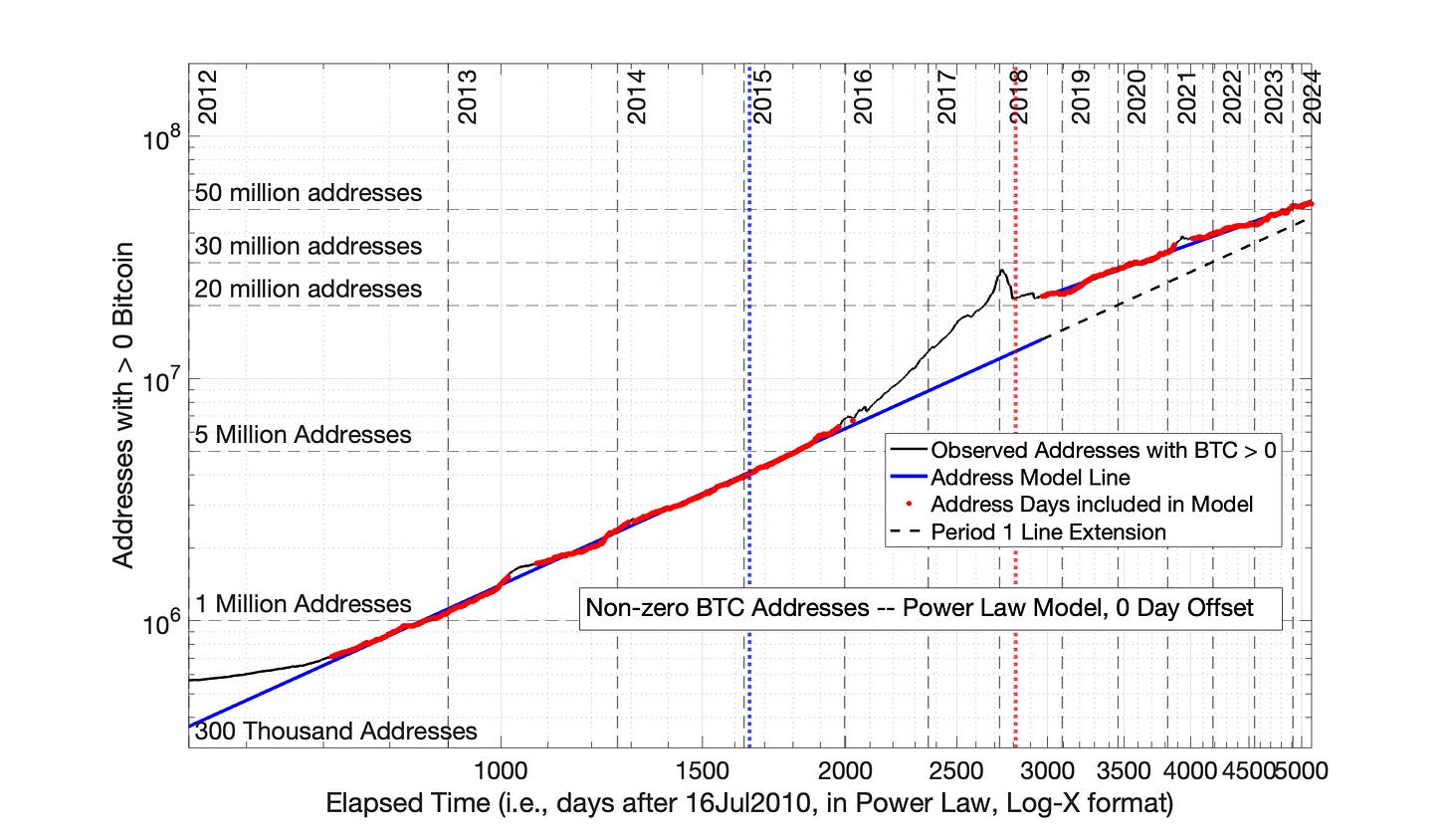
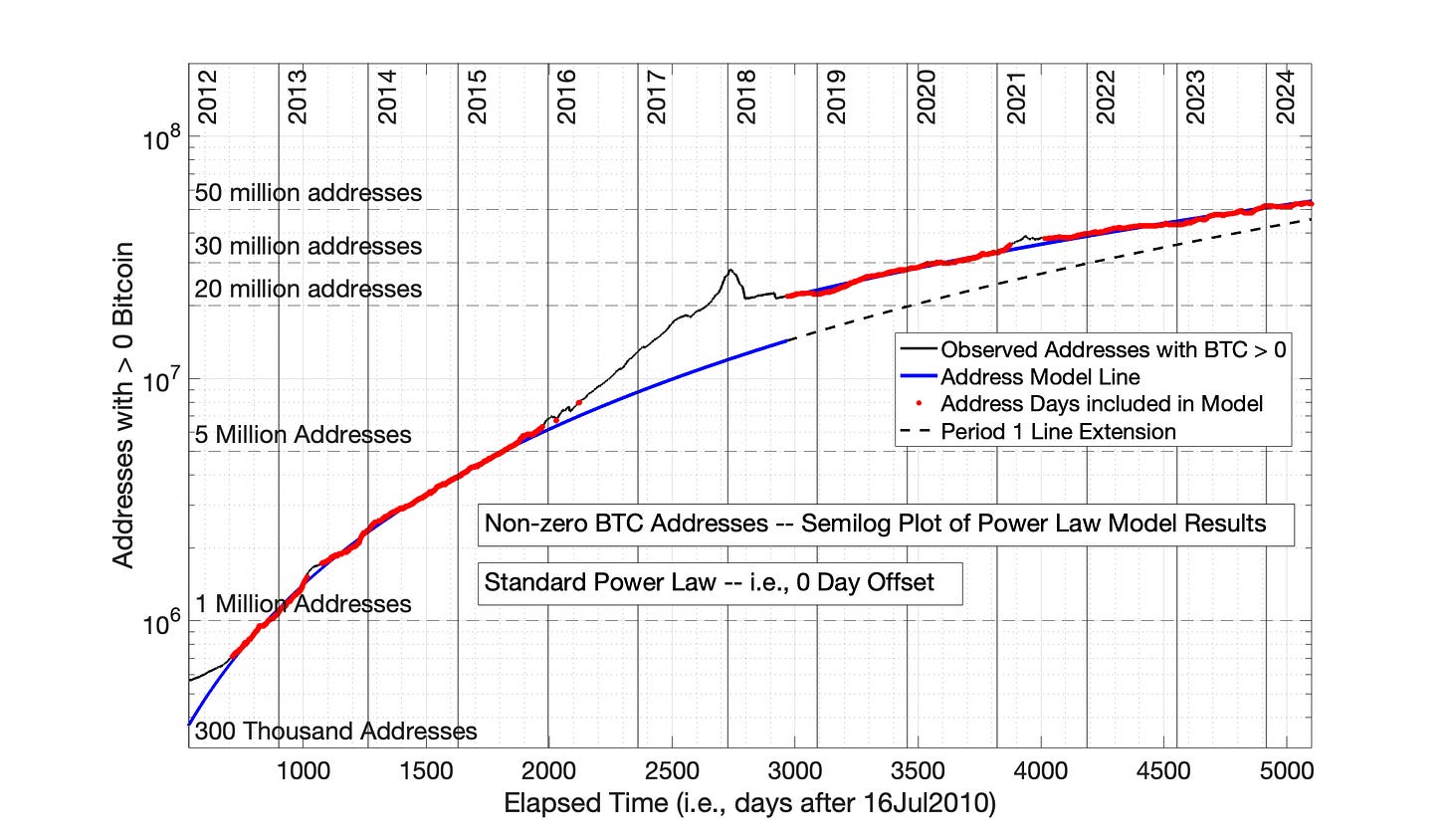
Fig 8.5 reveals that the modeling of Bitcoin adoption by the Power Law with 0-day offset falls into the same category as the seven technology adoptions presented in Chapter 7. The Power Law (with 0 time offset) has over-adjusted the early data too far to the right, as shown pictorially is Fig 7.1 The impact of the Power Law with 0 time offset on Period 1 and 2 data in Fig 8.5 resembles the impact observed for Periods 1 and 2 of Fig 7.19. When the Power Law results from Fig 8.5 are converted back to a semilog plot in Fig 8.6, a significant disconnect between Periods 1 and 2 is observed — similar to the disconnect between Period 1 and 2 data in Fig 7.20.
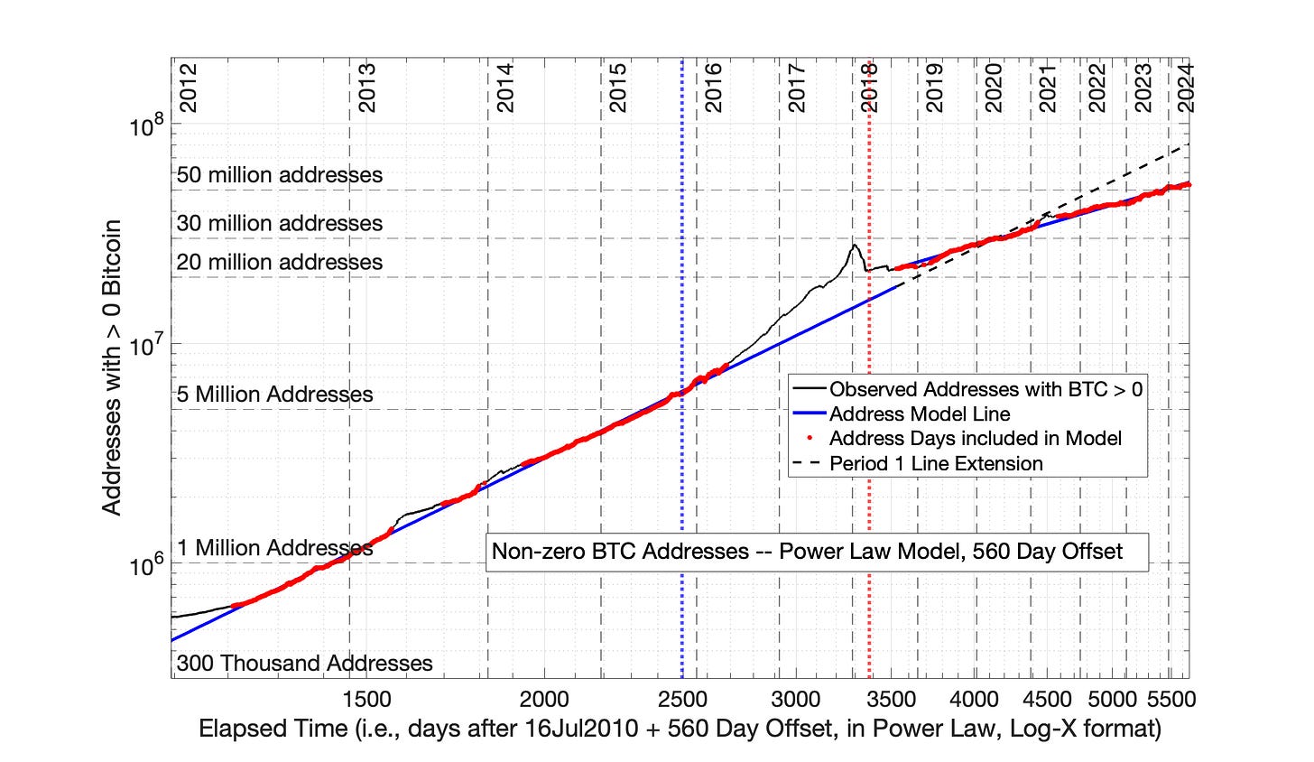
A time offset of 560 days results in transitional plots (Figures 8.16 and 8.17). The Power Law over-adjustment of data has been weakened, but there is still a disconnect between the data in Period 1 and Period 2 observed in both Figures 8.7 and 8.8. At an offset of 560 days, the Power Law is still over-adjusting the data points to the right.
The addition of a time offset of 2000 days in Fig 8.9 eliminates the data discontinuity between Periods 1 and 2, the clearest indication that the Power Law with this offset is appropriately representing the data. This result is reminiscent of results presented in Chapter 7.
The time offset of 2000 days also brings the Power Law results very close to alignment with SRET model results of Fig 8.3. When the Power Law model equations from Fig 8.9 are converted to semilog format in Fig 8.10, the results are nearly identical to the semilog plot of Fig 8.4 generated from SRET model results. That is, a time offset of 2000 days ( 5.5 years) is necessary to bring the Power Law into alignment with the SRET model results, and both models are appropriately representing the data under these circumstances.
Fig 8.5 Bitcoin-Containing Addresses: the Power Law model with 0 day time offset. Bitcoin-containing addresses are evaluated by the Power Law model (0 time offset) in 2 periods: Period 1: from 01Jan2012 to 01Sep2018 and Period 2: from 01Sep2018 to 01Jul2024. Explanation of the graph features is the same as Fig 8.3. The disconnect between the 1st and 2nd periods is consistent with Power Law over-adjustment of data to the right (as shown pictorially in Fig 7.1). The modeling of Bitcoin-containing addresses falls into the category of the historic technology adoptions of Chapter 7. The R2 for Periods 1 and 2 were 0.999 and 0.995, respectively.
Fig 8.6. Bitcoin-containing cddresses: Power Law model results from Fig 8.5 (no time offset) are plotted semilog versus time. The results are consistent with Power Law over-adjustment of data, consistent with the technology adoptions of Chapter 7.
Fig 8.7 Bitcoin-containing addresses: Power Law model with 560 day (1.5 year) time offset. Bitcoin-containing addresses are evaluated by the Power Law model (560 day time offset) in 2 periods: Period 1: from 01Jan2012 to 01Sep2018 and Period 2: from 01Sep2018 to 01Jul2024. Explanation of the graph features is the same as Fig 8.3. The 560 day time offset has weakened the over-adjustment of data points by the Power Law, but there is still a disconnect between the first and second periods. These results are consistent with the scenarios demonstrated in Chapter 7 — the time offset is not yet of sufficient magnitude. The R2 for Periods 1 and 2 were 0.999 and 0.995, respectively.
Fig 8.8. Bitcoin-containing cddresses: Power Law model results from Fig 8.7 (560 day time offset) are plotted semilog versus time. The results are consistent with Power Law over-adjustment of data, with a time offset which is insufficient.
Fig 8.9 Bitcoin-containing addresses: Power Law model with 2000 Day (5.5 year) time offset. Bitcoin-containing addresses are evaluated by the Power Law model (2000 day time offset) in 2 periods: Period 1: from 01Jan2012 to 01Sep2018 and Period 2: from 01Sep2018 to 01Jul2024. Explanation of the graph features is the same as Fig 8.3. The 2000 day time offset is sufficient to: 1) eliminate the disconnect between Periods 1 and 2; and 2) bring this figure into alignment with the SRET Model (Fig 8.3). The R2 for Periods 1 and 2 were 0.999 and 0.994, respectively.
Fig 8.10. Bitcoin-containing addresses: Power Law model results from Fig 8.9 (2000 day time offset) are plotted semilog versus time. The 2000 day time offset is sufficient to: 1) eliminate the disconnect between Periods 1 and 2; and 2) bring this figure into alignment with the SRET Model (Fig 8.4).
8.5 The Post-2018 Downward Shift in Adoption Rate is also Observed for other Glassnode Bitcoin Address Categories.
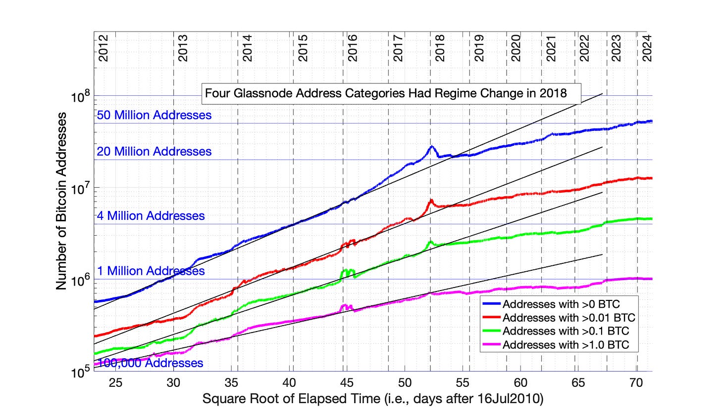
The post-2018 regime reduction in Bitcoin network size growth is observed for three other Bitcoin address categories from Glassnode (Fig 8.11).
Fig 8.11. Three Other Bitcoin Glassnode Address Categories Reveal a Downshift in Adoption Rate in 2018. The three categories are: 1) Addresses with > 0.01 BTC; 2) Addresses with > 0.1 BTC; and 3) Addresses with > 1 BTC.
8.6 A Downward Shift in Adoption Rate for Bitcoin Self-Custody Holders also Occurs after 2018.
The category of Bitcoin-containing addresses includes Bitcoin held by large entities (for example, Coinbase and Fidelity), as well as individuals who self-custody their own Bitcoin. The on-chain analysis company Glassnode has determined an approach to interrogate the Bitcoin address data to separate out the Bitcoin owned by large entities. This is the concept of “forensic clustering” of Bitcoin address information.
On 06Jun2023, the on-chain analysis pioneer Willy Woo presented a Twitter post in which the history of forensically-clustered, Bitcoin self-custody owners was shared. (https://x.com/woonomic/status/1666121983959142400). (data originating from Glassnode)
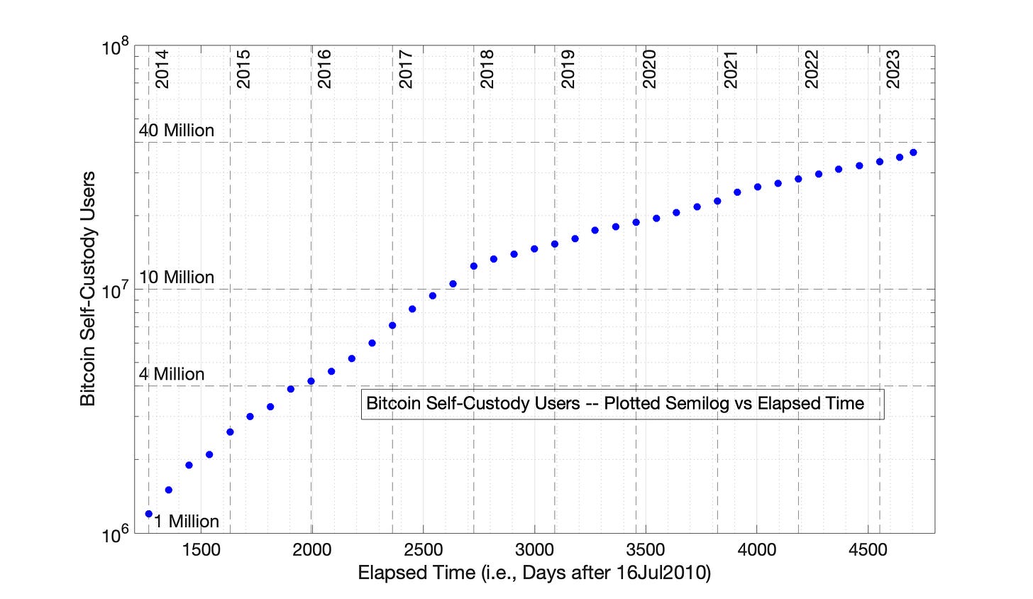
I digitized this data (Fig 8.12). These data show an obvious downturn in adoption rate in 2018. I then analyzed this data by both the Square Root of Elapsed Time (SRET) model and the Power Law Model, assuming two adoption periods. The detailed results of this analysis, which mirrored Sections 8.3 and 8.4, are presented in the Appendix.
The results of this analysis mirrored the results from Sections 8.3 and 8.4.
There was a downturn in adoption rate in 2018
A time offset of 2000 days was needed to bring the Power Law model into alignment with the SRET model.
Fig 8.12. Semilog plot of Bitcoin self-custody owners vs time, 01Jan2014 to 01Jun2023 Bitcoin Address Data from the Glassnode, Forensically-Clustered Analysis of Self-Custody Bitcoin owners was plotted semilog vs elapsed time. Data is digitized from a post of Bitcoin modeling pioneer Willy Woo. (https://x.com/woonomic/status/1666121983959142400)
8.7 Detailed Chapter 8 Conclusions
1. The Power Law model with time offset was introduced in Chapter 7. The time offset is not often mentioned explicitly in conjunction with the Power Law model, but its use is implicit in the establishment of Day 1 for the adoption data. For example, the true Day 1 of Bitcoin price and market cap history is 17Jul2010. But, the most popular “Twitter” application of the Power Law for Bitcoin recasts Day 1 as Jan 3, 2009. The actual Day 1 becomes Day 561 in this new Twitter Bitcoin model formulation.
In this Substack, Bitcoin Day 1 is maintained as 17Jul2010, and the popular Bitcoin model noted above has a time offset of 560 days — the is, the Power Law model equation for the popular Twitter Bitcoin model is:
ln(N) = n*ln(elapsed time + 560) + d.
2. An analysis of Bitcoin network size adoption in Chapter 8 provides clear evidence that Bitcoin network size adoption rate experienced an adoption regime change in 2018. For the self-custody user count data presented in the Appendix, the 2018 regime change was evident in the semilog plot versus time (Fig 8.12), and was further clarified by SRET model (Fig 8.13) and the Power Law model, with 0 offset (Fig 8.15), 560 day time offset (Fig 8.17) and 2000 day time offset (Fig 8.19). This 2018 regime change is probably obvious to many people in the semilog lot versus time of Bitcoin-containing address data (Fig 8.1), but this 2018 shift is absolutely clear in the SRET model analysis (Fig 8.3) and the Power Law analysis with 2000 day time offset (5.5 years, Fig 8.9).
3. In contrast, the analysis of Bitcoin-containing address count by the Power Law with time offsets of 0 days and 560 days produced plots consistent with Power Law data over-adjustment, like the 7 historic technology adoptions of Chapter 7. The Power Law (time offset of 0) resulted in a significant discontinuity between Periods 1 and 2 (Figures 8.5 and 8.6). This result is consist with heightened data adjustment in the 2nd quadrant of the original semilog plot of adoption data of Fig 8.1, resulting in a Period 1 plot in Fig 8.5 that is over-adjusted to the right. The time offset of 560 days reduced the data discontinuity between Periods 1 and 2, but did not eliminate it.
Note 1: The Power Law time offset of 560 days (~1.5 years) corresponds to the value used by Giovanni Santostasi for his version of Bitcoin Power Law model (“The Bitcoin Power Law Theory,”, Medium.com, 30Mar2024. That is, Day 1 of his version of the Power Law is 3Jan2009, 560 days before the first day of Bitcoin price history in the Glassnode database, 17Jul2010, which was Day 1 in the analyses in these Substack chapters.
Note 2. It is most productive to NOT associate the Power Law time offset with a specific date in history. The Power Law time offset is just a mathematical adjustment to the Power Law formula to reduce over-adjustment of data points — for example, a Power Law time offset of 4 years reduces length of the red arrows of Fig 7.1 to the blue arrows in that figure.
8.8. Data Sources and Analysis
Bitcoin network data in this chapter are provided by the cryptocurrency analysis provider Glassnode (www.glassnode.com), as part of an “Advanced” membership plan at about $30/month.
Day 1 of Bitcoin price and market cap history in the Glassnode database is 17Jul2010. The Glassnode daily market cap and Bitcoin-containing address counts are numbered from Day 1 through Day 5099 (July 1, 2024). The period of primary focus is Day 534 (01Jan2012) to Day 5099.
Data analyses and preparation of figures were performed using Matlab (www.mathworks.com).
8.9 References
Metcalfe, B. Metcalfe’s Law after 40 Years of Ethernet. Computer, 46(12): 26-31, 2013.
Alabi, K. Digital blockchain networks appear to be following Metcalfe’s Law. Electronic Commerce Research and Applications, 24: 23-29, 2017.
Peterson, TF. Metcalfe’s Law as a model for Bitcoin’s value, Alternative Investment Analyst Review, 7:9-18, 2018.
Van Vliet, B. An alternative model of Metcalfe’s Law for valuing Bitcoin. Economic Letters, 165: 70-72, 2018.
Alabi, KA. 2020 perspective on ‘Digital blockchain networks appear to be following Metcalfe’s Law’. Electronic Commerce Research and Applications, 40: 100939, 2020.
8.10 About the Author
The author has a B.S. and PhD. In chemical engineering. His PhD thesis focussed on mathematical modeling, simulation, and implementation of process control. Following his PhD, he was a university professor for 10 years at two US universities, focusing on both research and teaching. At both universities he taught the required chemical engineering course in process modeling and control. He subsequently spent more than 20 years in industrial chemical engineering practice.
8.11 Appendix - SRET Model and Power Law Model Analysis of Bitcoin Self-Custody Holders
An alternative source of Bitcoin network size information was provided in a 06Jun2023 Twitter (‘X’) post by on-chain analysis pioneer Willy Woo (https://x.com/woonomic/status/1666121983959142400). The data associated with this tweet was a plot of “forensically-clustered” Bitcoin self-custody owners as a function of time (data originating from Glassnode).
The on-chain analysis company Glassnode has stated their ability to use forensic observations of on-chain address data to identify which Bitcoin addresses belong to exchanges (such as Coinbase) and which Bitcoin addresses are assigned to individual users. The latter group are termed “forensically-clustered” Bitcoin self-custody owners.
I digitized the data set presented in Willy Woo’s email. Fig 8.12 is a semilog plot of forensically-clustered Bitcoin self-custody owners as a function of time, from 01Jan2014 to 01Jun2023. The dates are numbered based on a Day 1 of 17Jul2010. By this convention, the 01Jan2014 and 01Jun2023 are Days 1265 and 4703, respectively. This semilog plot of Fig 8.12 makes no assumption of any modeling approach. A transition from “Period 1” to “Period 2” is evident in 2018.
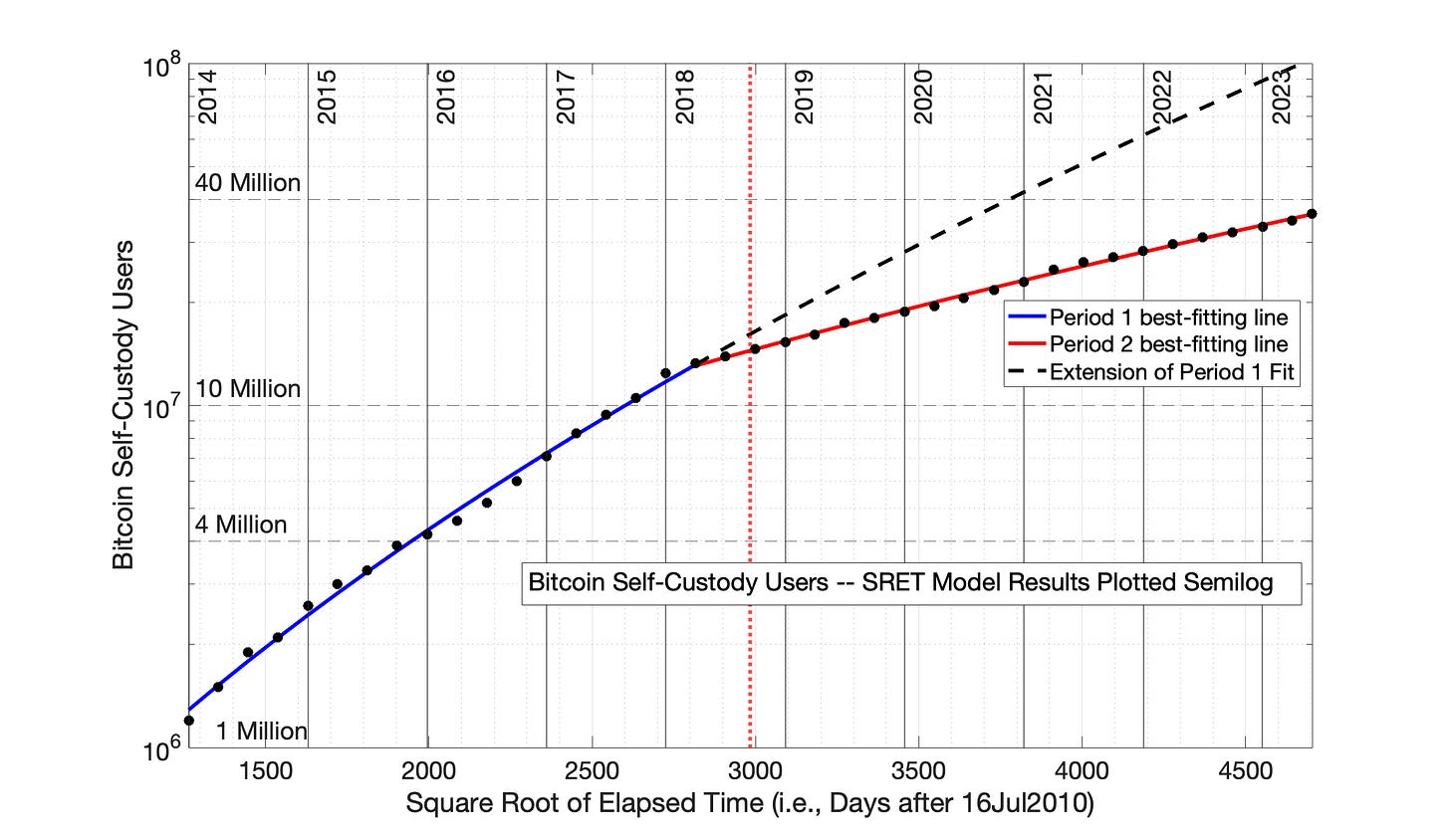
The data from Fig 8.12 is replotted in the Square Root of Elapsed Time model format in Fig 8.13. These data reinforce the observation of a change in regime starting in 2018. The blue and red, best-fitting straight lines in Fig 8.4 have the model formulas
“Blue” Period 1: ln(N) = 0.1327*(sqrt of elapsed time) + 9.349
“Red” Period 2: ln(N) = 0.06575*(sqrt of elapsed time) + 12.90
where N is the Self-custody user count. Sqrt and * are the symbols for square root and multiplication, respectively.
The black dashed line in Fig 8.13 is a simple extension of Period 1 model equation into Period 2, providing a visual perspective on the change in adoption rate between Periods 1 and 2.
The blue and red, vertical, dotted lines in Fig 8.13 have the same meaning as in Chapters 6 and 7. The dotted red line represents the temporal midpoint of the data — the midpoint in time. The dotted blue line represents the visual midpoint of the data. The difference between these two lines is a measure of time distortion created by the SRET Model in order to linearize the adoption data — that is, expansion of earlier time periods and compression of later time periods.
In Fig 8.14, the model equations from Fig 8.13 are plotted semilog versus time along with the original data (i.e., no time distortion), demonstrating the rapid but decelerating growth typical of technology adoptions.
Fig 8.13. Bitcoin self-custody owners, 01Jan2014 to 01Jun2023: Square Root of Time (SRET) Model. The data from Fig 8.12 was plotted in the SRET Model format, and least-squares, best-fitting straight lines were determined for blue and red, Periods 1 and 2. The dashed black line is the extrapolation of the Period 1 SRET model into Period 2, to provide a visual perspective on the decline in adoption rate in Period 2. The vertical, dotted red line represents the temporal midpoint of data presented on the x-axis, while the vertical, dotted blue line represents the visual midpoint of the x-axis data. The R2 for Periods 1 and 2 were 0.996 and 0.998, respectively.
Fig 8.14. Bitcoin self-custody owners, SRET Model equations from Fig 8.13 plotted semilog versus time. The data and SRET model equations demonstrate the rapid, but decaying growth rate typical of technology adoptions. Also typical of technology adoptions is the organization of the adoption data into distinct adoption periods — the blue and red lines. A dashed, black line is provided to change in adoption rate occurring between Periods 1 and 2. By convention, Day 1 of Bitcoin price history is 17Jul2010.
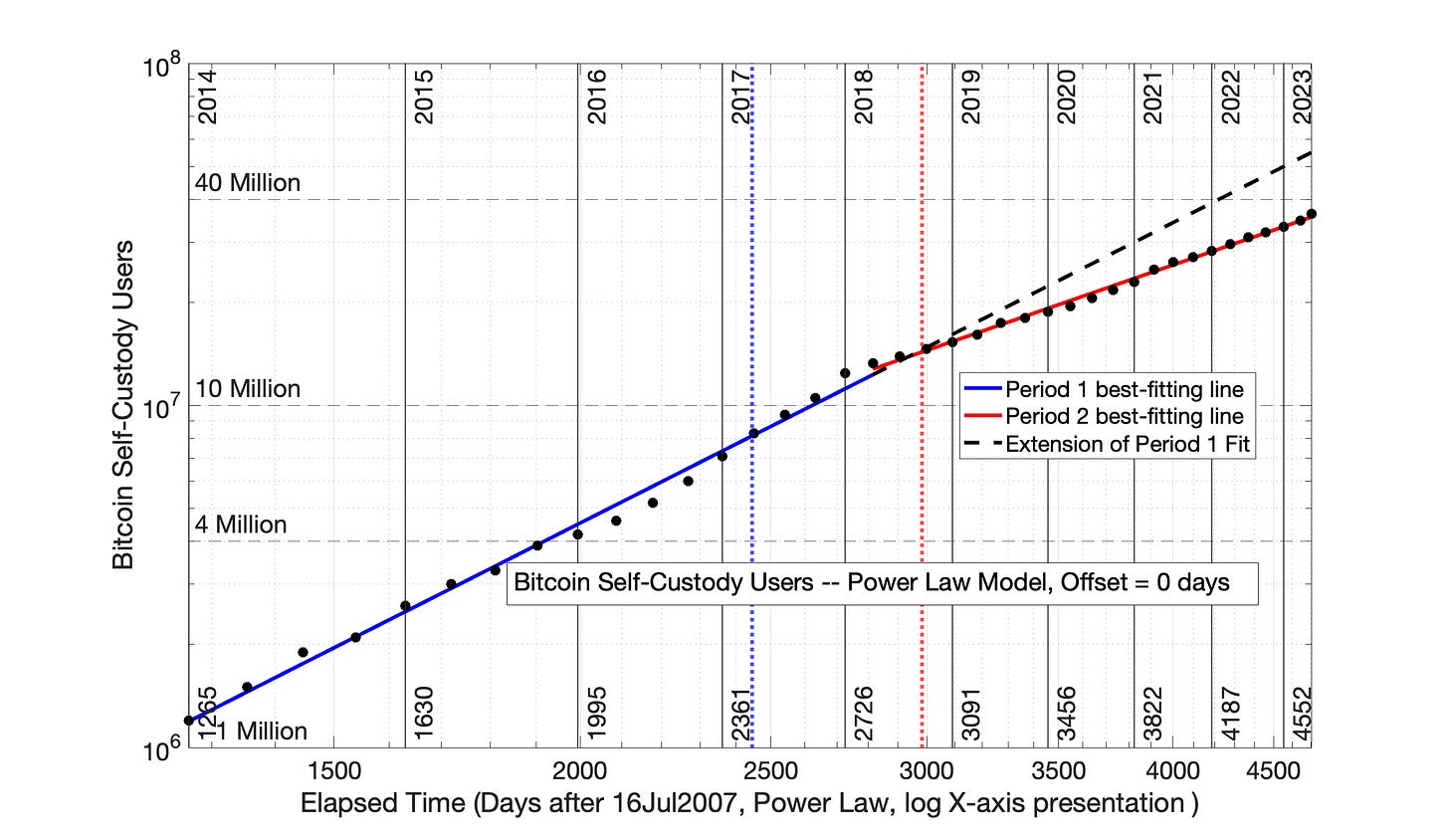
This Glassnode self-custody data was then plotted using the Power Law model with 0 time adjustment (Fig 8.15). This plot is consistent with a regime change in 2018.
The blue and red, best-fitting straight lines in Fig 8.15 have the model formulas
“Blue” Period 1: ln(N) = 2.916*ln(elapsed time) - 6.841
“Red” Period 2: ln(N) = 1.995*ln(elapsed time) + 0.5149
where N is the Self-custody user count. Ln and * are the symbols for natural logorithm and multiplication, respectively.
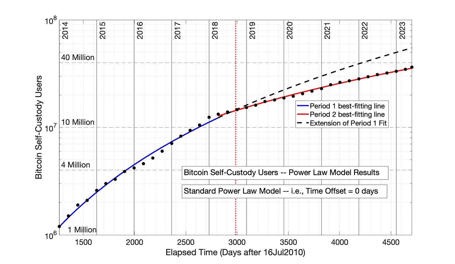
The original data and Power Law model equations from Fig 8.15 are plotted semilog versus time in Fig 8.16.
Fig 8.15 Bitcoin self-custody owners, 01Jan2014 to 01Jun2023: Power Law model with 0 time offset. The data from Fig 8.12 was plotted in the Power Law format, and least-squares, best-fitting straight lines were determined for blue and red, Periods 1 and 2. The vertical, dotted red line represents the temporal midpoint of data presented on the x-axis, while the vertical, dotted blue line represents the visual midpoint of the x-axis data. By convention, Day 1 of Bitcoin price history is 17Jul2010. The R2 for Periods 1 and 2 were 0.993 and 0.996, respectively.
Fig 8.16 Bitcoin self-custody owners, Power Law model equations from Fig 8.15 plotted semilog versus time. The data and Power Law model equations demonstrate the rapid, but decaying growth rate typical of technology adoptions. Also typical of technology adoptions is the organization of the adoption data into distinct adoption periods — the blue and red lines. A dashed, black line is the extension of the Period 1 model equation into Period 2, providing to visualize the decline in adoption rate between Periods 1 and 2.
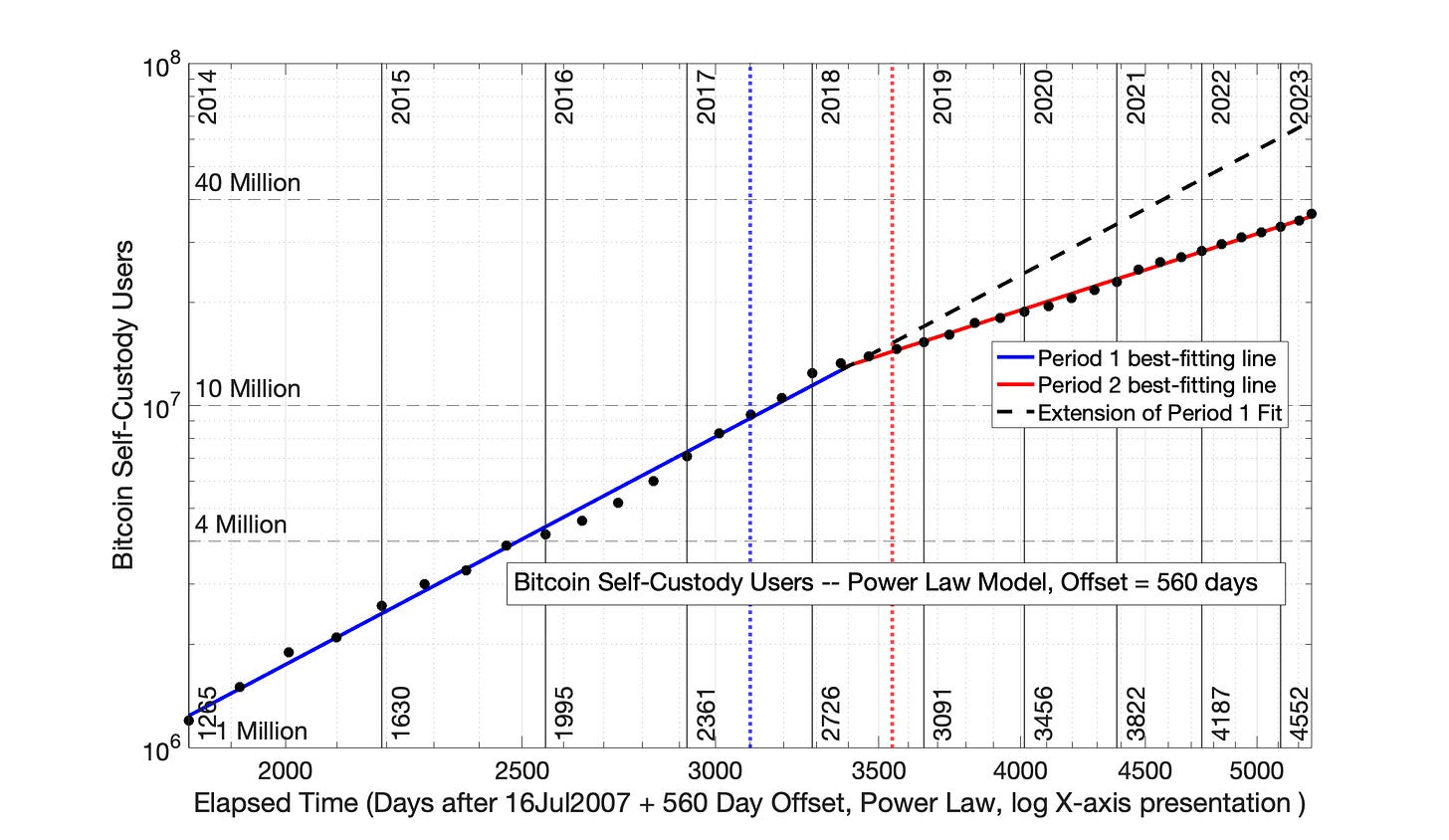
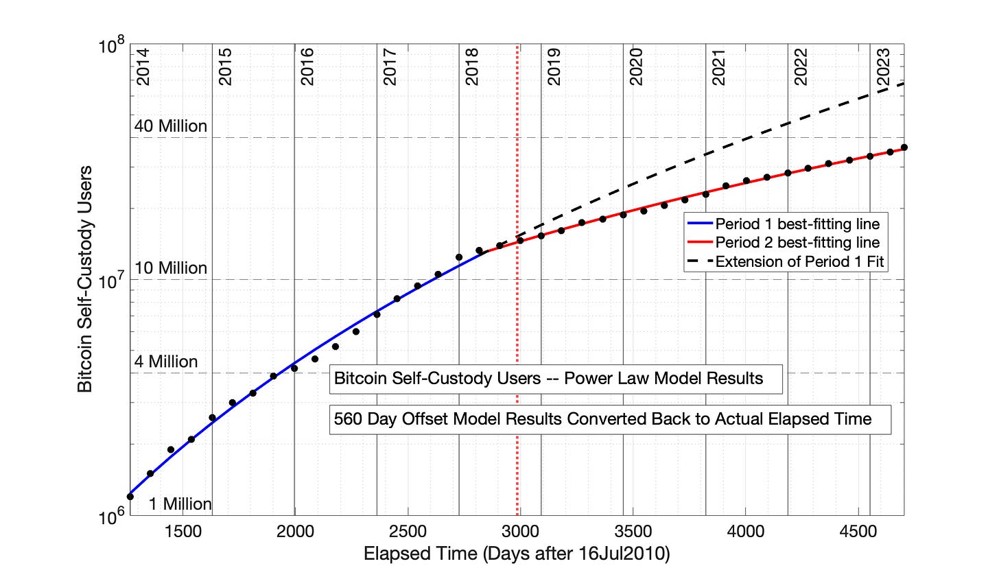
As established in Chapter 7, the solution to excess time distortion by the Power Law model with 0 time offset is the addition of a time offset. Two time offsets were explored, 560 days and 2000 days — See Figures 8.17 and 8.19, respectively.
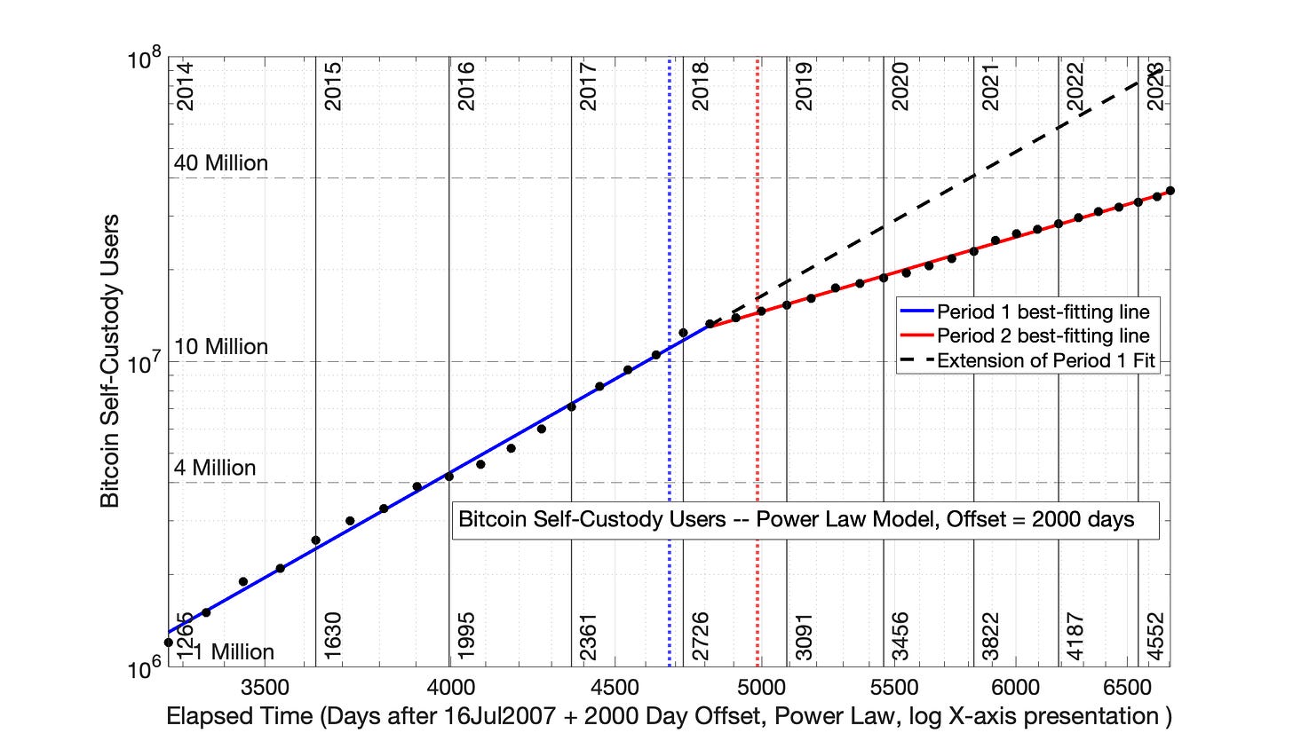
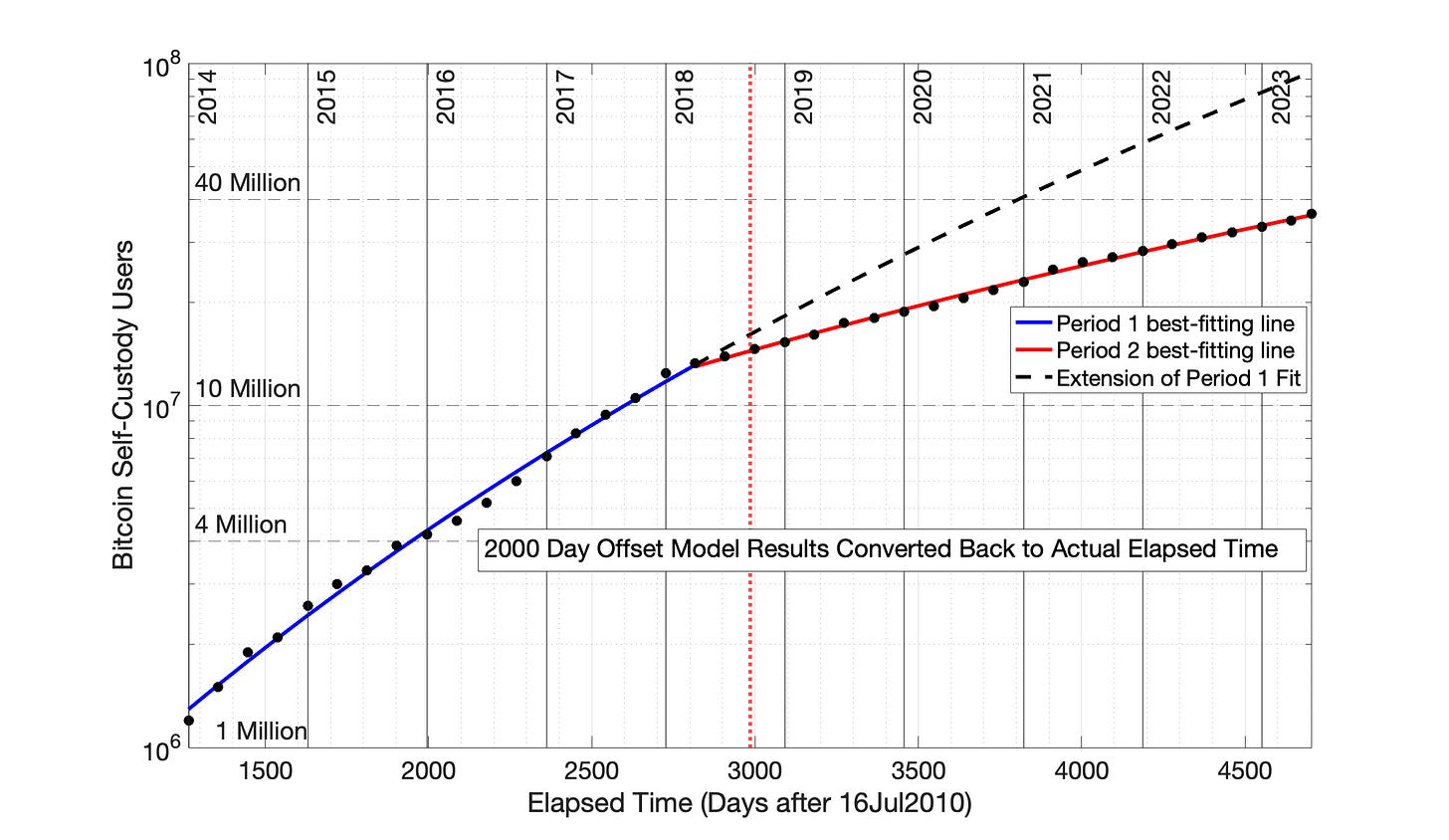
The Power Law model with 2000 day time offset yields results more closely aligned with the SRET Model — compare Figures 8.19 and 8.20 with Figures 8.9 and 8.10. The distance between the vertical, dotted blue and red lines in Figures 8.9 and 8.19 are also comparable, indicating comparable levels of time distortion in the two figures.
Fig 8.17 Bitcoin self-custody owners, 01Jan2014 to 01Jun2023: Power Law model with 560 day (1.5 Year) time offset. The data from Fig 8.12 was plotted in the Power Law format, and least-squares, best-fitting straight lines were determined for blue and red, Periods 1 and 2. The R2 for Periods 1 and 2 were 0.995 and 0.997, respectively.
Fig 8.18 Bitcoin self-custody owners, Semilog plot of the Power Law model equations from Fig 8.17. The data and Power Law model equations demonstrate the rapid, but decaying growth rate typical of technology adoptions. Also typical of technology adoptions is the organization of the adoption data into distinct adoption periods — the blue and red lines. A dashed, black line is the extension of the Period 1 model relationship into Period 2, provided to visualize the reduction in adoption occurring between Periods 1 and 2.
Fig 8.19 Bitcoin self-custody owners: Power Law model with 2000 day (5.5 year) time offset. The data from Fig 8.3 was plotted in the Power Law format, and least-squares, best-fitting straight lines were determined for blue and red, Periods 1 and 2. The R2 for Periods 1 and 2 were 0.996 and 0.998, respectively. These results resemble the SRET model results of Fig 8.13.
Fig 8.20 Bitcoin self-custody owners: Power Law model equations from Fig 8.19 (time offset of 2000 days, 5.5 years) plotted semilog versus time. The data and Power Law model equations demonstrate the rapid, but decaying growth rate typical of technology adoptions. These results with a 2000 day offset resemble the SRET model results of Fig 8.14.
The blue and red, best-fitting straight lines in Fig 8.17 have the model formulas
“Blue” Period 1: ln(N) = 3.780*ln(elapsed time + 560) - 14.36
“Red” Period 2: ln(N) = 2.302*ln(elapsed time + 560) - 2.332
The blue and red, best-fitting straight lines in Fig 8.19 have the model formulas
“Blue” Period 1: ln(N) = 5.961*ln(elapsed time +2000) - 34.16
“Red” Period 2: ln(N) = 3.086*ln(elapsed time +2000) - 9.786
The presentation of the model formulas above is primarily to remind the reader of the meanings of the Power Law time offset.

