Chapter 7. Modeling technology adoptions of the 20th and 21st century: Part 2. When the Power Law Model Fails
The Power Law model and the SRET model are applied to seven more technology adoptions. The Power Law model (with 0 time offset) fails to properly identify adoption periods.
7.1 Overview/Summary
Seven historic technology adoptions of the 20th and 21st century were analyzed in Chapter 6 using both the Power Law and SRET models. In all seven cases, both models were successful in linearizing the adoption data to identify distinct adoption periods.
During each adoption period, technology adoption is marked by rapid growth, but with a decelerating annual growth rate. That is, the native adoption data in a semilog plot (like Fig 6.2) are inherently concave. The Power Law and SRET approaches are effective in “linearizing” adoption data by distorting the position of the data on the X-axis, expanding the width of earlier time periods and contracting the width of later time periods.
In Chapter 7, seven additional historic technology adoptions are explored in which the Power Law model with 0 time adjustment does NOT appropriately linearize the technology adoption data. Chapter 7 does provide guidance for adjustment/modification of the Power Law model time offset to successfully linearize data for the seven technology adoptions.
The Bitcoin network is in the same category of the seven historic technology adoptions described in Chapter 7 — a non-zero time adjustment is required for the Power Law. So, it is particularly important to take the time to understand the content and implications of Chapter 7. Modeling of the Bitcoin network will begin in Chapter 8.
The seven examples presented in Chapter 7 are:
Worldwide Adoption of Facebook (as measured by Network Size), 2004 to 2015
US Adoption of Home Refrigeration, 1931 to 1956
US Cell Phone Adoption, 1994 to 2019
US Adoption of Home Telephone, 1903 to 1942
US Adoption of Color Television, 1966 to 1989
US Adoption of Home Radio, 1925 to 1948
US Adoption of the Automobile, 1915 to 1954
One of the interesting aspects of 14 historic technology adoptions reviewed in Chapters 6 and 7 is the similarity of technology adoption profiles across the 20th and 21st centuries. The major difference between the 20th and 21 century technology adoptions was the impact of the Great Depression and World War II on technology adoption from 1927 to 1945. But, apart from this tumultuous period, diverse technology adoptions appear to follow a repeatable pattern.
7.2 The Power Law model with 0 time adjustment can over-adjust data points.
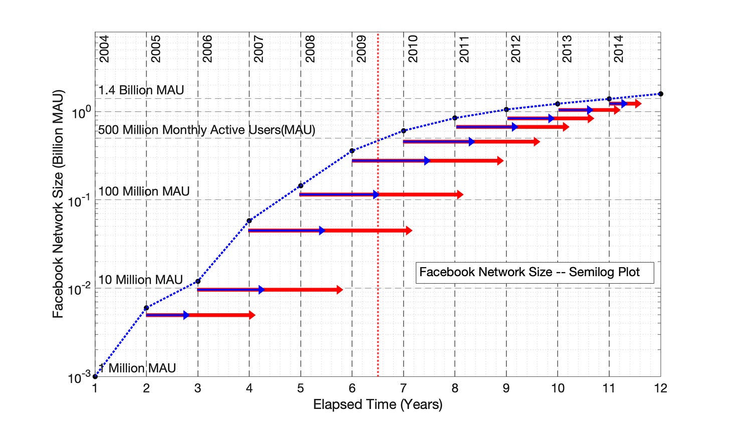
The worldwide adoption of Facebook social media between 2004 and 2015 is presented as a semilog plot in Fig 7.1, measured as the growth of monthly active users with time. This plot demonstrates the concave shape typical of technology adoptions — rapid but decelerating growth.
A good way to understand how the SRET model and Power Law model function is to create a semilog of adoption data (Fig 7.1), and monitor the length that each data point is translocated to a SRET model plot (Fig 7.2) or a Power Law model plot (Fig 7.4)
Fig 7.1 includes blue arrows showing the adjustment of individual data points by the SRET model to create Fig 7.2, and red arrows demonstrating the adjustment of individual data points by the Power Law model to create Fig 7.4.
Overall, the Power Law model (with 0 time offset) is twice as powerful as the SRET model in data translocation — that is, the red arrows in Fig 7.1 are twice the length of the blue arrows (Figures 7.1, 7.2 and 7.4).
Differential movement of data points by the SRET and Power Law models is essential for linearization of the curved adoption data of Fig 7.1. The greatest graphical movement between Figures 7.1 and 7.2/7.4 is by the Year 4 and 5 data points, followed by the Year 3, 6 and 7data points, followed by the Year 2, 8 and 9 data points, followed last by the year 10 and 11 data points. In essence, the greatest SRET model and Power Law model data translocation is to the 2nd quadrant of adoption data, followed by the 1st and 3rd quadrants, and finally by the 4th quadrant.
Vertical, dotted, vertical, blue and red lines in the figures of Chapters 6 through 9 provide a measure of the degree of data shift in each graph. The dotted, vertical red line represents the temporal midpoint of the graph, which the dotted blue line represents the visual midpoint of the graph. The distance between these lines is a measure of the time distortion created by the SRET model to linearize the adoption data.
The dotted blue lines in Fig 7.1 connect the individual data points to highlight the visual appearance of this typical semilog technology adoption curve.
Fig 7.1 International Facebook Adoption, 2004 to 2015: Semilog Plot of Network Growth. Monthly active users (MAU) on the y-axis is the measure of network size. Blue and red arrows indicate the point-specific shift of data when plotted in the SRET model (Fig 7.2) or Power Law model with 0 time offset (Fig 7.4), respectively.
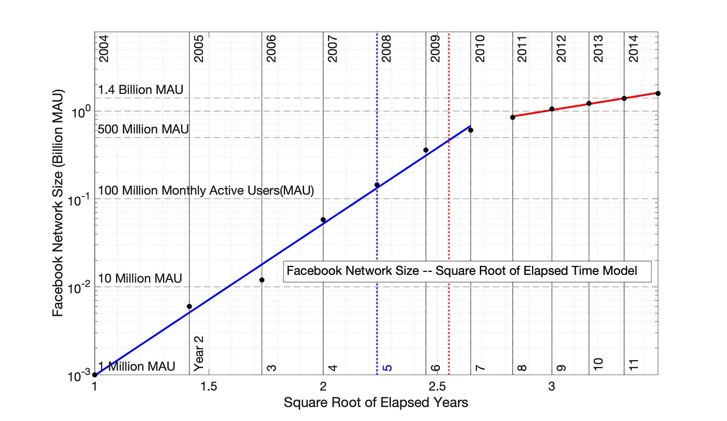
Figure 7.2 represents application of the Square Root of Elapsed Time (SRET) model to the Facebook network size data of Fig 7.1. Numbers on the x-axis are the square root of each adoption year.
The SRET model is successful in linearizing the data, and identifying 2 discrete adoption periods. The solid, blue and red lines through these periods are the equations:
“Blue”, Period 1: ln(network size) = 3.977*(square root of elapsed time) - 10.907
“Red”, Period 2: ln(network size) = 0.9734*(square root of elapsed time) - 2.894
Where ln and * are the symbols for natural log and multiplication, respectively.
The slopes 3.977 and 0.9734 of these two equations are the adoption rates of these periods. A four-fold decline in adoption rate (3.977/0.9734) occurred between Years 7 and 8 (2010 to 2011) of the Facebook network adoption.
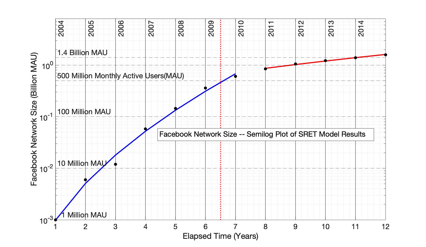
Fig 7.3 presents the SRET model equations in semilog format — that is, the linear, SRET model equations of Fig 7.2 are converted back into the “time” domain in Fig 7.3, demonstrating the excellent fit of the model to the original data.
Fig 7.2 International Facebook adoption, 2004 to 2015: Application of the Square Root of Elapsed Time (SRET) model. The vertical, dotted red line represents the temporal midpoint of data presented on the x-axis, while the vertical, dotted blue line represents the visual midpoint of the x-axis data. R2 values of “blue” and “red” Periods 1 and 2 are 0.993 and 0.991, respectively.
Fig 7.3 International Facebook adoption, 2004 to 2015: SRET model results from Fig 7.2 are presented as a semolina plot. The identify of the two, linear blue and red period of Fig 7.2 are shown in this semilog plot of adoption data. There is no time distortion on the x-axis, so the vertical, dotted blue and red lines of Fig 7.2 condense into a single red, dotted line in this figure.
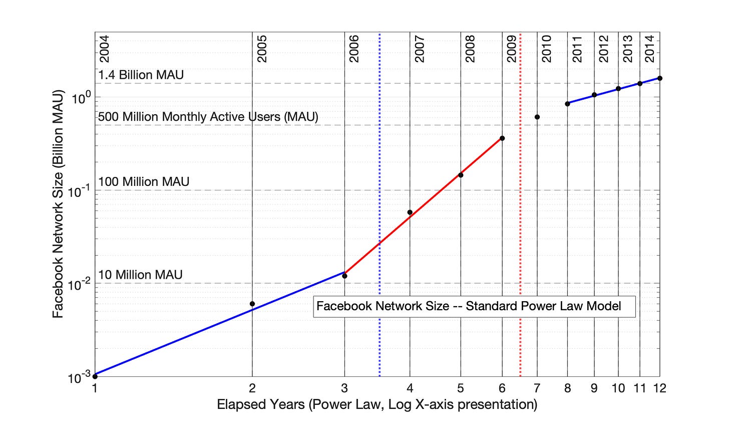
In Fig 7.4, the Power Law model is applied to the Facebook adoption data. The Power Law model with 0 time offset is more intense than the SRET model in terms of time distortion, as judged by Fig 7.4 and the relative sizes of the red and blue arrows in Fig 7.1 .
Application of the Power Law model (with 0 time offset) has “over-adjusted” the data points to the right in Fig 7.4. The concave shape of Year 1 to 6 data of Fig 7.1 has been over-adjusted into a convex shape Fig 7.4. The single, “blue” period of the SRET model (Fig 7.2) has become two initial periods in Fig 7.4. That is, these first two periods are the artifact of the Power Law over-adjustment of time.
Fig 7.5 presents the Facebook Power Law model equations in semilog format — that is, the 3 linear, Power Law model equations of Fig 7.4 are converted back into the “time” domain in Fig 7.5 to show the fit of the model to the original data.
Fig 7.4 International Facebook adoption, 2004 to 2015: Power Law model with 0 time offset. The data set is from Fig 7.1. The Power Law has over-adjusted the concave, Year 1-6 adoption data of Fig 7.1 into a convex shape, represented by the first blue and red adoption periods. The vertical, dotted red line represents the temporal midpoint of data presented on the x-axis, while the vertical, dotted blue line represents the visual midpoint of the x-axis data. The distance between the blue and red, dotted lines is a measure of the time distortion of the Power Law (compare with Fig 7.2). The R2 values of the blue, red and blue lines are 0.990, 0.997 and 0.995, respectively.
Fig 7.5 International Facebook adoption, 2004 to 2015: Power Law model results from Fig 7.4 are presented as a semilog plot. The identify of the 3 adoption periods of Fig 7.4 are shown in this semilog plot of adoption data. There is no time distortion on the x-axis, so the vertical, dotted blue and red lines of Fig 7.4 condense into a single red, dotted line in this figure.
7.3 There is a mathematical fix to the Power Law time over-adjustment problem.
The problem with application of the Power Law with 0 time offset to many technology adoptions is the over-adjustment of the time axis. There is a relatively simple fix to this problem — appropriate selection of a positive, non-zero time offset . Prior to application of the Power Law model, the data set is adjusted by adding a number of additional years to the elapsed time for each data point in the series — the “Power Law Time Offset”.
The abbreviated, original data set for Figures 7.1 through 7.5 is:
Year Year Number Monthly Active Users (Billion MAU)
2004 1 0.001
2005 2 0.006
2006 3 0.012
……………………………………………………………………………...
2013 10 1.228
2014 11 1.393
2015 12 1.591
After a Power Law time adjustment of 4 years, the new data set is:
Year Year Number Monthly Active Users (Billion MAU)
2004 5 0.001
2005 6 0.006
2006 7 0.012
……………………………………………………………………………...
2013 14 1.228
2014 15 1.393
2015 16 1.591
The Power Law model equation is
ln(Facebook network size) = n*ln(elapsed time + f ) + d (Fig 7.6)
Where f is a positive constant. In this example, f = 4 years.
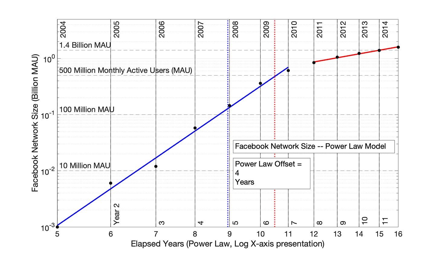
The Power Law model with an offset of 4 years is plotted as Fig 7.6. The data from 2004 to 2010 has been linearized. The distance between the vertical red and blue dotted lines of Fig 7.4 have been narrowed to be similar to the SRET model (Fig 7.2), indicating less time distortion on the x-axis.
If Fig 7.5 was converted to a semilog plot, the resulting plot would look like Fig 7.3.
Fig 7.6 International Facebook adoption, 2004 to 2015: Power Law Model with Data Offset of 4 Years. The convexity of the plotted data in Fig 7.4 is “fixed” by adding 4 years to each time point in the series before application of the Power Law model. This adjustment is displayed at the difference between the x-axis values and adoption years inside the graph. The R2 values of the blue and red adoption periods are 0.993 and 0.993.
7.4 The Problem with Power Law Modeling of Technology Adoption
In Section 7.3, addition of a “time adjustment factor” to the Power Law model was shown to “correct” the time over-adjustment of the Power Law model.
In some cases, we will know that the Power Law model is not optimally optimized if there is a clear discontinuity between adoption periods. However, in Figures 7.4 and 7.5 there is not clear evidence of discontinuities at the intersection of adoption periods.
We only knew the Power Law model with 0 time adjustment had over-adjusted time (Fig 7.4) because of a comparison to SRET model results (Fig 7.2). Without the SRET model results as reference, we would not know whether Fig 7.4 or 7.6 was correct.
The full implication of the Facebook network example is that the Power Law may sometimes be be unsuitable for independently identifying technology adoption periods. This conclusion is explored in the following six examples.
Looking ahead: Fortunately, in the Power Law modeling of Bitcoin market size and market cap, the optimal choice of time offset is evident in both: 1) the disappearance of discontinuities at period boundaries and 2) a match to SRET model results.
7.5 Another Example of the Power Law Modeling Problem: US Adoption of Home Refrigeration
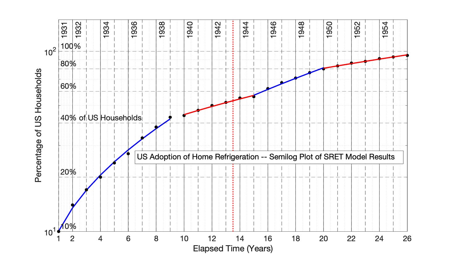
The SRET model of US adoption of home refrigeration is presented in Fig 7.7. Four linear adoption periods are identified. The second, adoption period covers the period of World War II and probably represents a war-induced constraint on adoption of this technology. The SRET model results are replotted in semilog format in Fig 7.8.
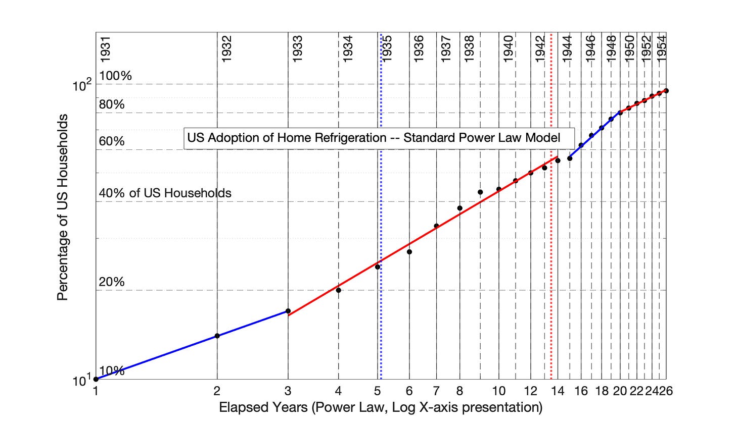
In Fig 7.9, the Power Law model (with no time adjustment) is applied to the US Home Refrigeration data. The higher intensity of the Power Law modeling approach has created a convex plot. The first and second periods of Fig 7.7 have been divided into two new adoption periods in Fig 7.9.
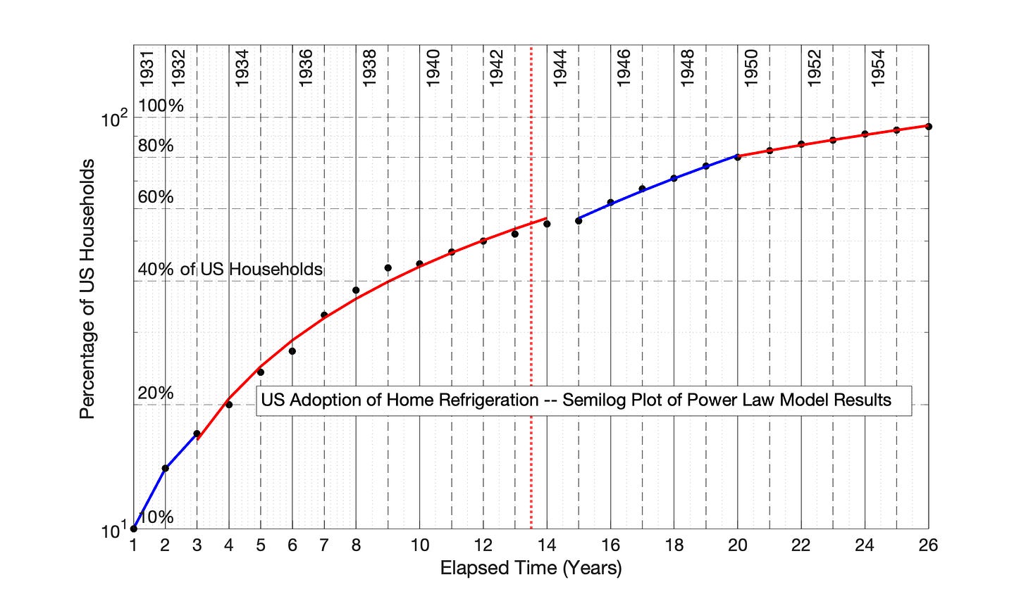
The Power Law model results are replotted semilog in Fig 7.10. The resulting plot displays humps and discontinuities not present in Fig 7.8.
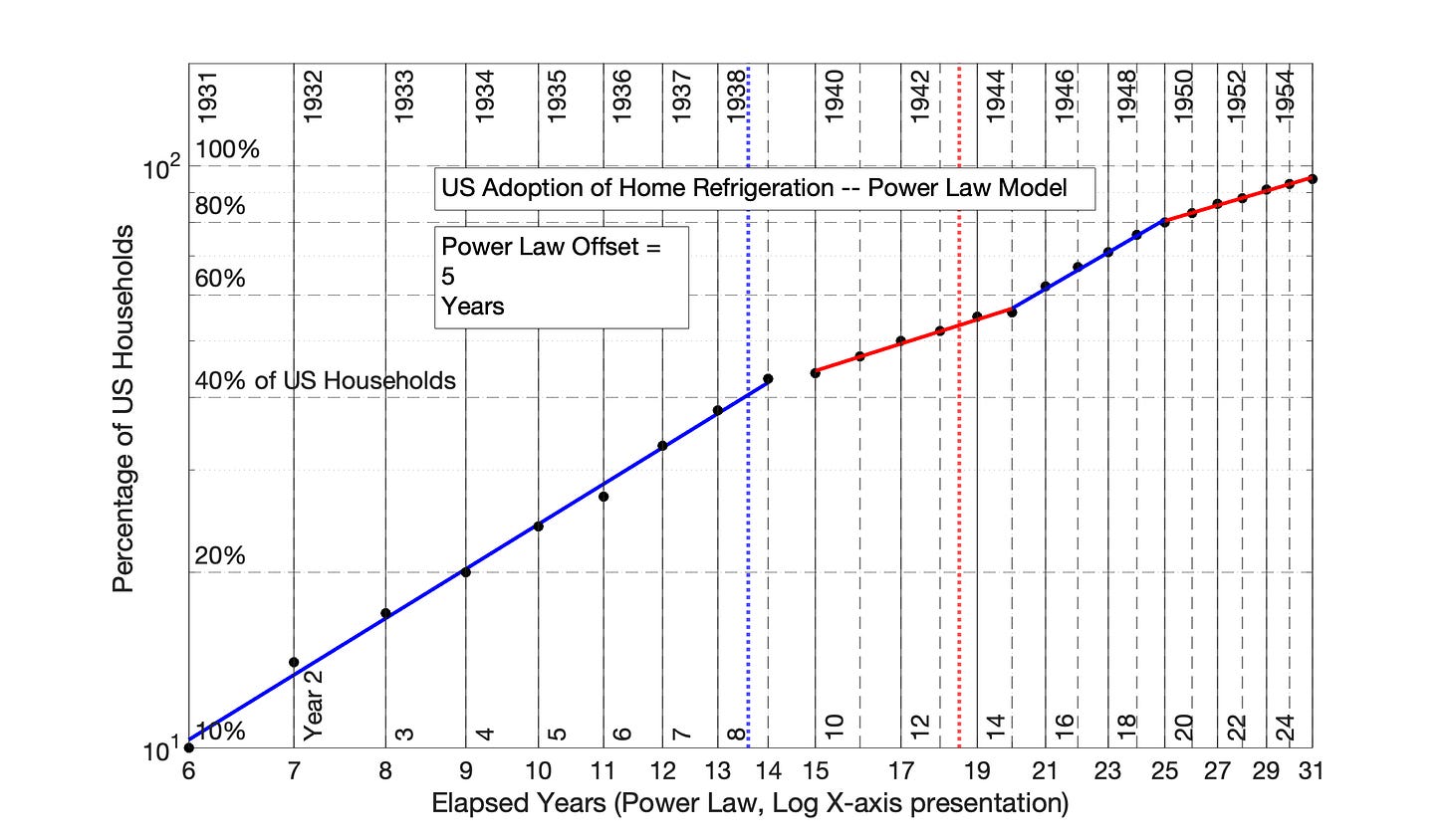
The Power Law model is corrected in Fig 7.11 by addition of a 5-year time offset to the data, analogous to the 4-year offset in Fig 7.6. After the 5-year offset, Fig 7.11 now resembles the SRET model results of Fig 7.7.
Fig 7.7 US Adoption of Home Refrigeration, 1931 to 1956: Application of the Square Root of Elapsed Time (SRET) model. R2 values of the four adoptions periods from left to right are 0.997, 0.984, 0.991, and 0.994.
Fig 7.8 US Adoption of Home Refrigeration, 1931 to 1956: SRET model results from Fig 7.7 are presented as a semilog plot. The identify of the four, linear blue and red periods of Fig 7.7 are shown in this semilog plot of adoption data. There is no time distortion on the x-axis, so the vertical, dotted blue and red lines of Fig 7.2 condense into a single red, dotted line in this figure.
Fig 7.9 US Adoption of Home Refrigeration, 1931 to 1956: Power Law model with 0 time offset. The Power Law has over-adjusted the initial dozen years of adoption data concave, Year 1-6 adoption data, creating new data groupings in the first two adoption periods. The R2 values of the four adoption periods, from left to right, are 0.9999, 0.990, 0.994 and 0.996.
Fig 7.10 US Adoption of Home Refrigeration, 1931 to 1956: Standard Power Law model results from Fig 7.9 are presented as a semilog plot. The identify of the 4 adoption periods of Fig 7.9 are shown in this semilog plot of adoption data. Discontinuities have appeared at the intersection of adoption periods not seen in Fig 7.8.
Fig 7.11 US Adoption of Home Refrigeration, 1931 to 1956: Power Law Model with time offset of 5 Years. The convexity of the plotted data in Fig 7.9 is “fixed” by adding 5 years to each time point in the series before application of the Power Law model. This adjustment is displayed at the difference between the x-axis values and adoption years inside the graph. The R2 values of 4 adoption periods, from left to right, are 0.996, 0.987, 0.993, and 0.995.
7.6 The Worst Case Scenario for the Power Law Problem
The Power Law problem that emerged in modeling Facebook network adoption (Figures 7.4 and 7.6) is repeated in the modeling of US of adoption of home refrigeration (Fig 7.9 and 7.11). In the absence of the SRET model results as a reference, there is no way of knowing which model interpretation is correct — Fig 7.4 or Fig 7.6 for the Facebook network adoption? Fig 7.9 or 7.11 for the adoption of US home refrigeration?
But, there is another, arguably worse scenario. A Power Law model of US adoption of home refrigeration with time offset of 1 year results in Fig 7.12. The one-year offset has created the appearance of a single adoption period extending for the full 26 years of data. The R2 of this fit is a solid 0.996.
It would be very tempting to misinterpret Fig 7.12 as the correct Power Law model fit.
Spoiler Alert: The scenario presented in Fig 7.12 will be repeated in the application of the Power Law model to Bitcoin market cap in Chapter 9.
Fig 7.12 US Adoption of Home Refrigeration, 1931 to 1956: Power Law Model with Time Offset of 1 Year Results in Data Misinterpretation. A suboptimal choice of the Power Law time offset results an unfortunate alignment of data. The adoption of home refrigeration is easily misinterpreted as occurring in a single adoption period on the basis of this graph. The R2 value of this incorrect adoption period is 0.996.
7.7 Additional Problematic Applications of the Power Law Model to Technology Adoption
Five more technology adoption examples are outlined in this section. The figures are found in the Appendix. The numbering system of the figures has been adjusted to make them easier to find and follow.
For example, for the US adoption of home telephone, the six figures are:
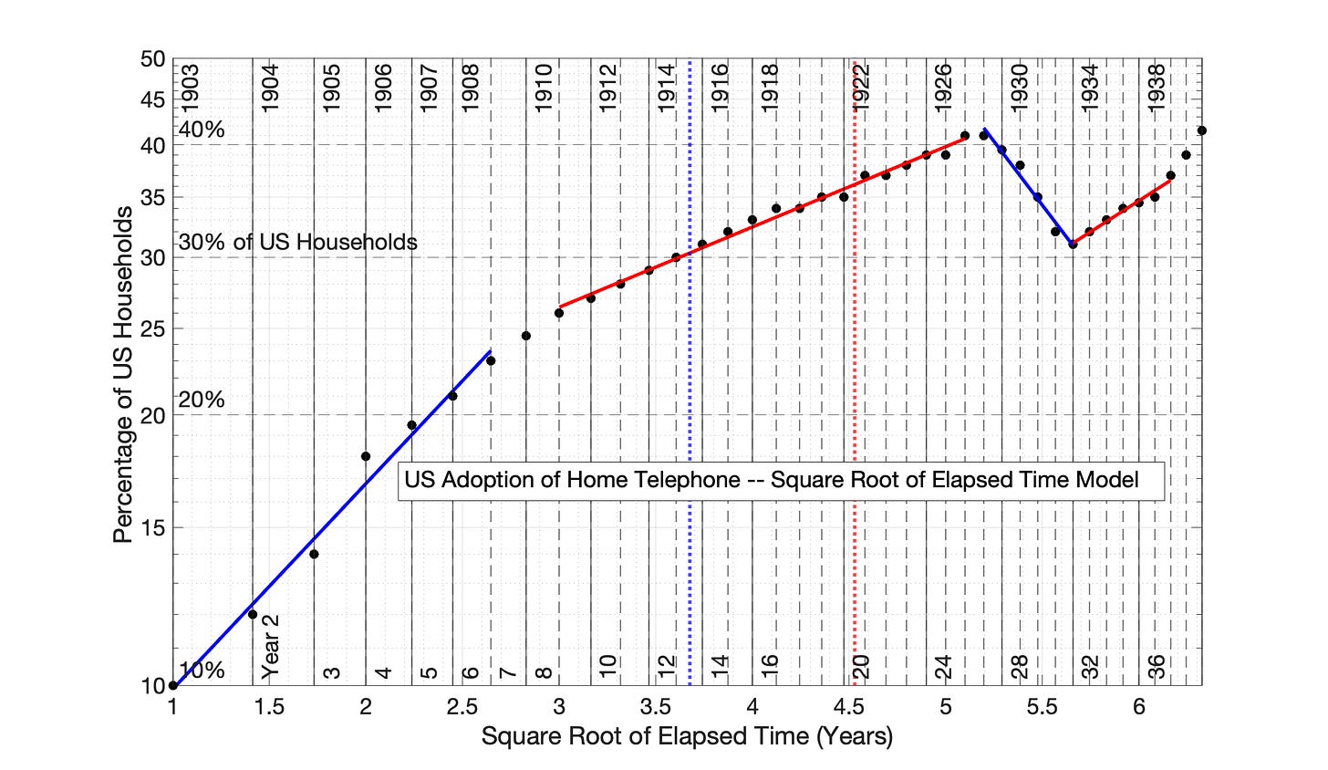
Fig 7.20 US Adoption of Home Telephone, 1903 to 1942: SRET model
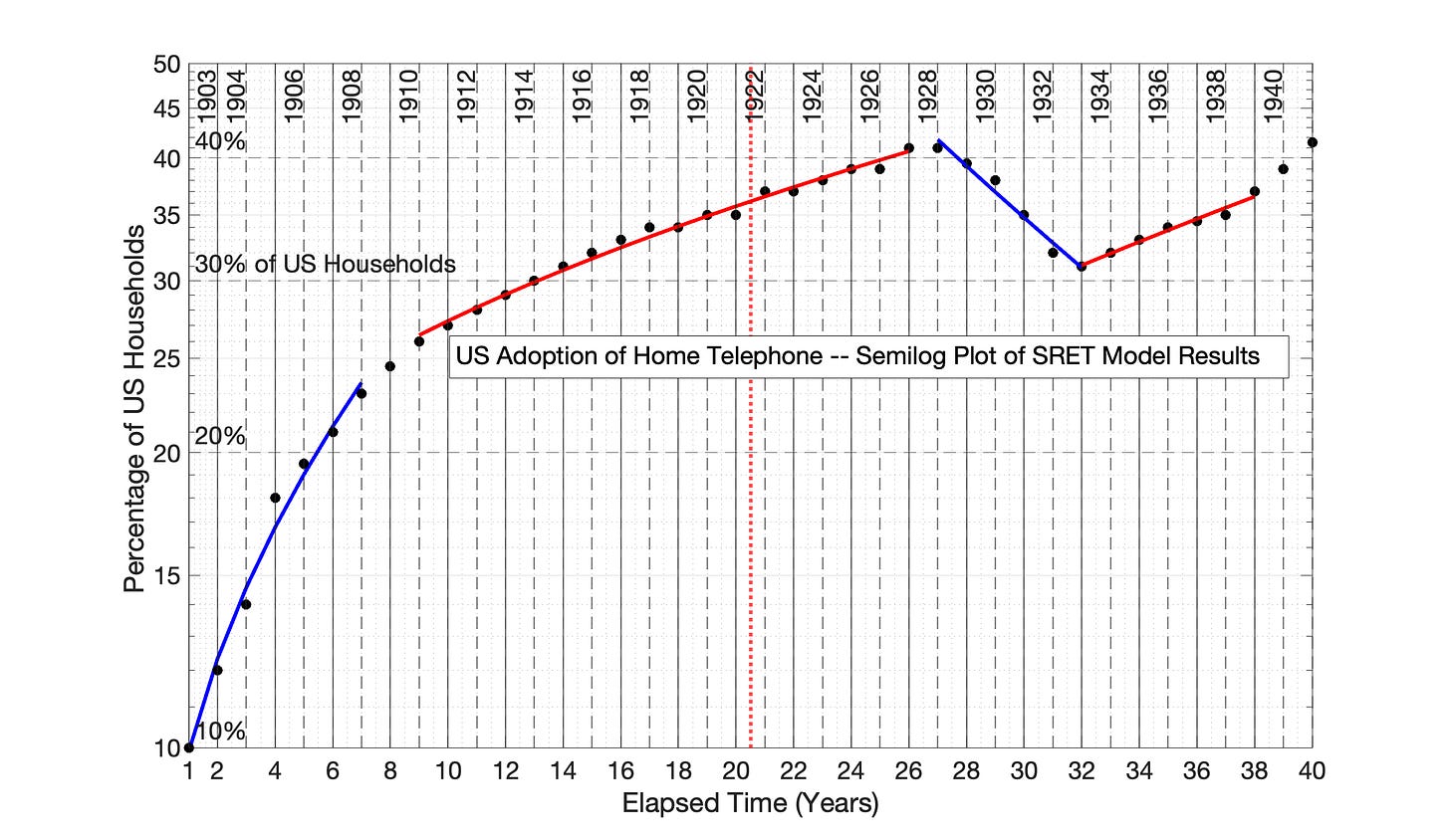
Fig 7.21 US Adoption of Home Telephone, 1903 to 1942: Semilog Plot of SRET Model Results
Fig 7.22 US Adoption of Home Telephone, 1903 to 1942: Power Law model (no time offset)
Fig 7.23 US Adoption of Home Telephone, 1903 to 1942: Semilog Plot of Fig 7.22 Power Law model Results (no time offset)
Fig 7.24 US Adoption of Home Telephone, 1903 to 1942: Addition of a 6-year Power Law time adjustment leads to a corrected Power Law plot.
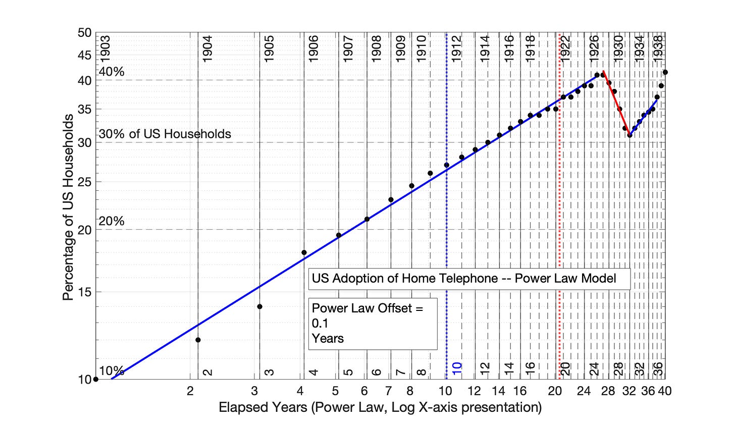
Fig 7.25 US Adoption of Home Telephone, 1903 to 1942: Addition of a 0.1-year Power Law time Aadjustment leads to Power Law plot that could be misinterpreted as linear for the first 26 years.
The same groupings of figures are also found in the Appendix for four other technology adoptions.
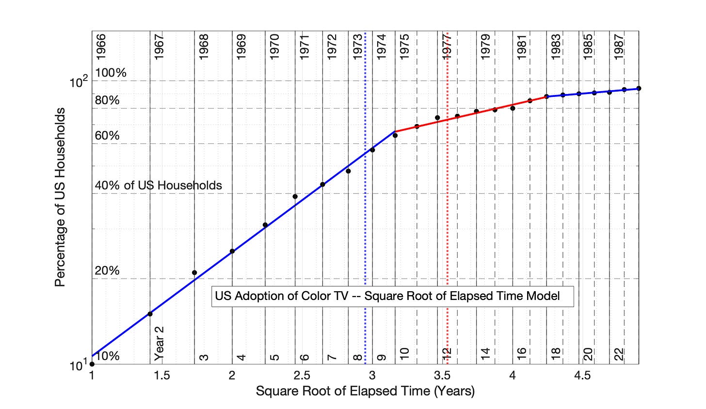
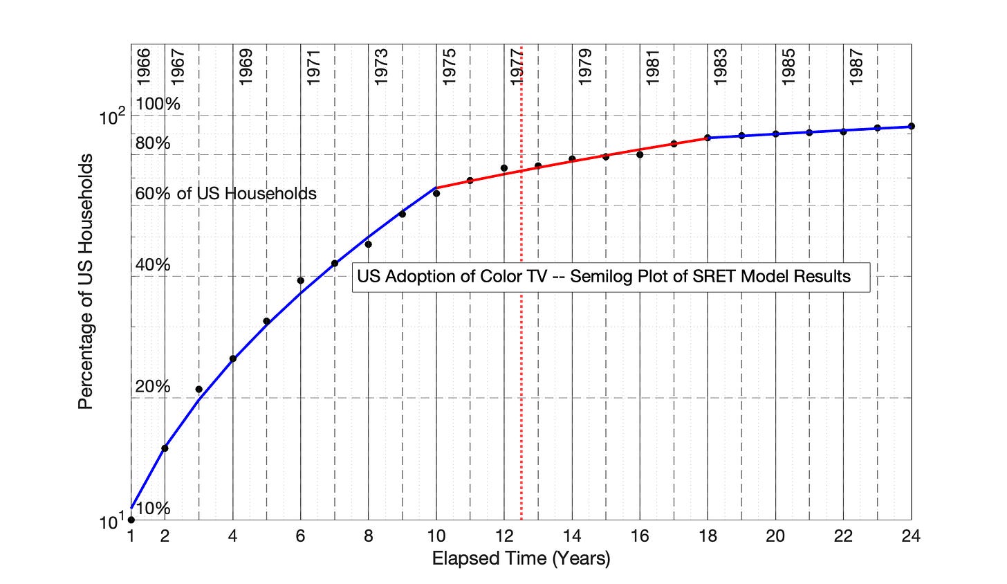
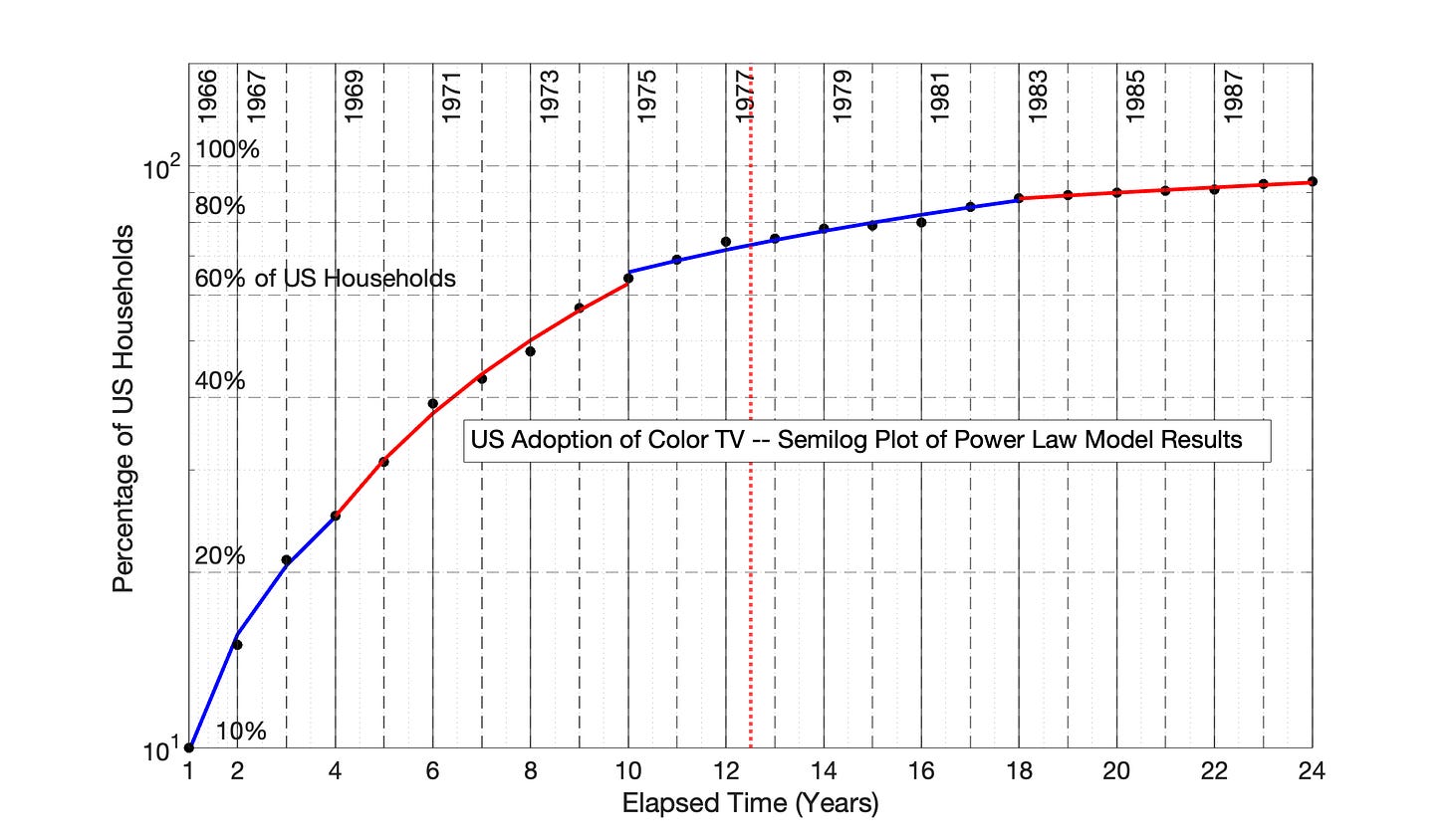
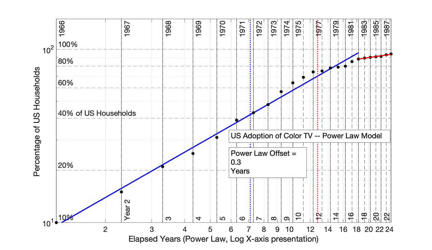
Figures 7.30 through 7.35: US Adoption of Color TV, 1966 to 1989
Figures 7.40 through 7.44: US Cell Phone Adoption, 1994 to 2019:
Figures 7.50 through 7.54: US Adoption of Radio, 1925 to 1948
Figures 7.60 through 7.64: US Adoption of the Automobile, 1915 to 1956
These results and their implications are discussed in Section 7.8
7.8 Detailed Summary of Results from Chapters 6 and 7
In this section, the analyses presented in Chapters 6 and 7 will be systematically presented. These results plus additional results from Chapters 8 and 9 lead to the conclusion of observation 22 that the popular Power Law model of Giovanni Santostasi presented frequently on Twitter is wrong.
that the popular “Twitter” model is based on a mis-tuned Power Law
that the presumption of this model that Bitcoin market cap has experienced a single period of linear growth is wrong. Bitcoin experienced a downshift in adoption rate for both network size and market cap in the 2018/2019 period.
To justify such strong statements, it is important to systematically present the observations/results leading to those conclusions. Below are the observations justified by the data in Chapters 6 and 7:
1. Fourteen historic technology adoptions have been analyzed in these Substack Chapters 6 and 7. All of these technology adoptions share a common form when plotted semilog as a function of time. They exhibit continuous, rapid growth, but with a decelerating annual growth rate.
2. The gold standard for any mathematical model of technology adoption is to find a mathematical formula that allows one to plot adoption data as a straight line — “a mathematical model that linearizes the data.” With such a mathematical formulation, technology adoption can be expressed as y = m*x + b, where m and b are the slope and intercept, respectively.
The Power Law model has the form
ln(N) = n*ln(elapsed time + time offset) + d
Where “ln” is the symbol for natural log, * is the multiplication symbol, and N is the symbol for network size (or network value). Time offset is a constant that must be optimized for each technology adoption.
The constants n and d are the slope and y-intercept, respectively.
This model is an excellent fit for any technology adoption data that plots as a straight line when plotted as ln(N) versus ln(elapsed time + time offset).
The formula for the Square Root of Elapsed Time (SRET) model is network size (or network value) is
ln(N) = m*(sqrt of elapsed time) + b,
Where “sqrt” is symbol for square root
The constants m and b are the slope and y-intercept, respectively.
This model is an excellent fit for any technology adoption data that plots as a straight line when plotted as ln(N) versus sqrt(elapsed time).
3. In spite of their different equation formats, the Power Law model and the SRET model are both capable of linearizing technology adoption data. This is demonstrated through analysis of 14 historic technology adoptions in Chapters 6 and 7.
4. A good way to understand how the Power Law and SRET models are achieving data linearization is to follow the movement of individual data points from a curved semilog adoption plot to a linearized format in a plot of the SRET model or Power Law model. This was the purpose of Section 7.2, Figures 7.1, 7.2 and 7.4. The Power Law model and the SRET model achieve their success by differentially moving the position of individual technology adoption points in time. Conceptually, consider the original adoption data (plotted semilog vs time, as in Fig 7.1) is divided into 4 quadrants — i.e., earliest 25% of data, next 25% of data, etc. Both the Power Law model and the SRET model move the data in the 2nd quadrant the most, followed by the 1st and 3rd quadrant, followed last by the 4th quadrant (Section 7.2.)
5. The standard Power Law model and the SRET model are not identical in their ability to linearize adoption data. In the example presented in Section 7.2, the standard Power Law moves individual data points almost twice the distance of the SRET model, as indicated by the blue and red arrows in Fig 7.1. This is also obvious in the comparison of Power Law model and SRET model plots for each of the 7 historic technology adoptions presented in Chapter 6 — e.g., compare Figures 6.2, 6.3 and 6.5. The Power Law model with 0 time offset is “more powerful” or “more intense” in its adjustment of technology adoption data points.
6. In spite of this difference in data-movement intensity, both the Power Law (with 0 time offset) and SRET models effectively linearize adoption data and identify the same technology adoption periods in the 7 historic technology adoptions of Chapter 6. The Power Law model (with 0 time offset) was clearly better than the SRET model for linearizing some adoption periods for the technology adoptions in Chapter 6 — for example, compare the 2nd, “red” period in Fig 6.3/6.4 (Power Law plots) with the same period in Fig 6.5/6.6 (SRET model plots). This superiority in linearizing an individual adoption period with strong curvature was repeated in 5 of the 7 technology adoptions of Chapter 6, as identified in Section 6.6.
7. For the 7 historic technology adoptions in Chapter 7, the SRET model was very effective in linearizing technology adoption data and identifying the proper adoption periods. That is, the SRET model was effective in identifying technology adoption periods in all 14 technology adoptions in Chapters 6 and 7.
8. The over-adjustment of data by the Power Law with 0 time adjustment is manifest for each of the 7 historic technology adoptions presented in Chapter 7. For example:
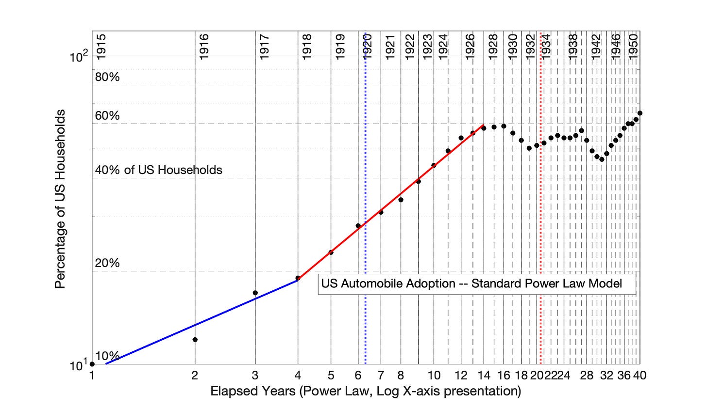
single adoption periods when plotted by the SRET model become two periods in a convex orientation when plotted by the Power Law model (compare Figures 7.2 and 7.4, 7.30 and 7.32, and 7.60 and 7.62).
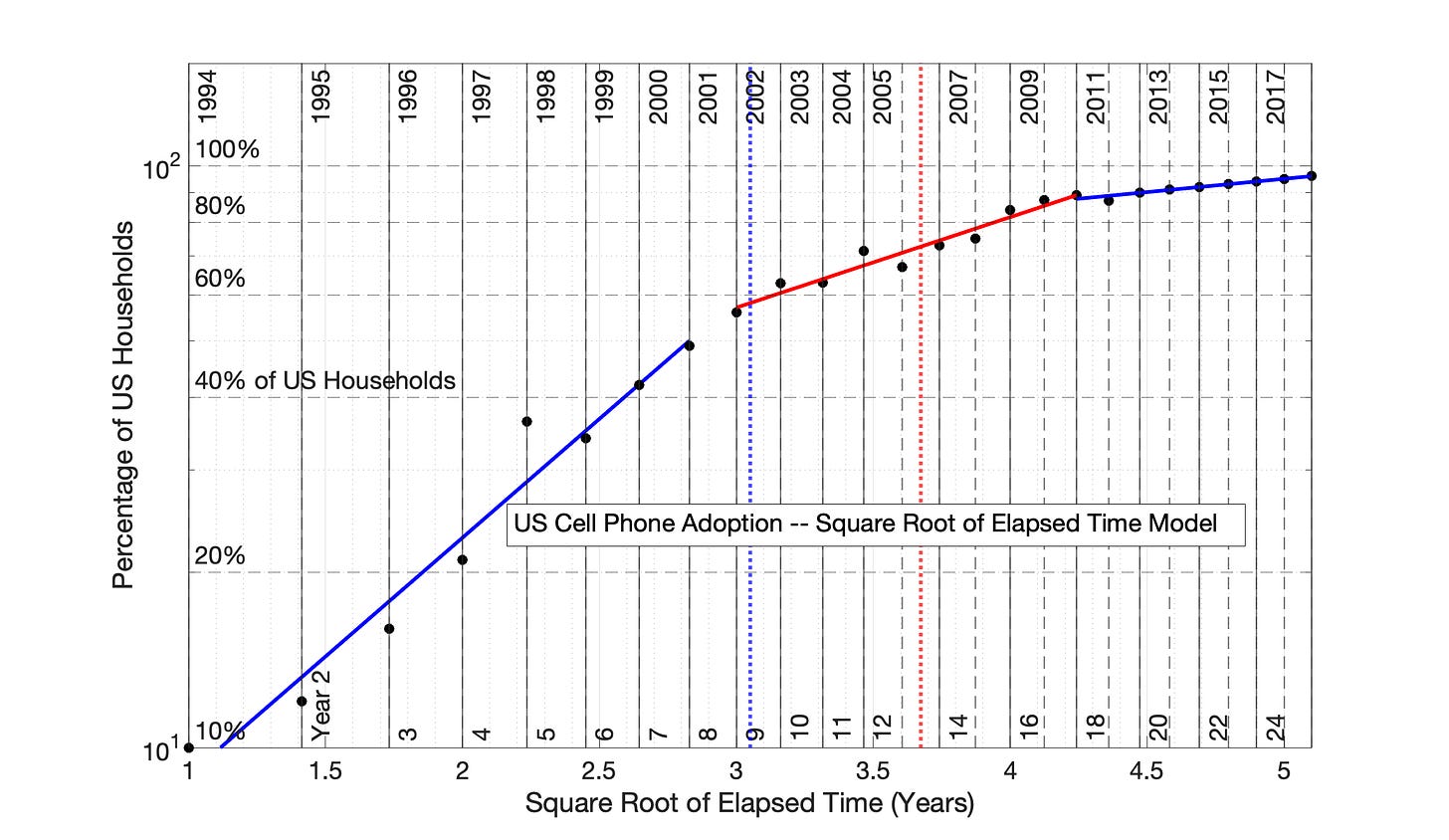
data points are rearranged into new adoption periods by the Power Law model (compare Figures 7.7 and 7.9; 7.20 and 7.22; 7.40 and 7.42; 7.50 and 7.52) and
discontinuity between adoption periods in the Power Law model (e.g., see Figures 7.22/7.23 and Fig 7.9/7.10).
9. The over-adjustment of data by the Power Law (with 0 time offset) in the Chapter 7 examples could be corrected in each case by identifying an optimal, positive time offset.
The Power Law with time offset was effective in linearizing the adoption data and identifying correct adoption periods for each of the 7 technology adoptions in Chapter 7 — for example, compare Figures 7.4 and 7.6, 7.9 and 7.11, 7.22 and 7.24, 7.32 and 7.34, 7.42 and 7.44, 7.52 and 7.54, and 7.62 and 7.64.
10. Thirteen of the 14 examples of Chapter 6 and 7 were chosen from a relatively small set of about 25 technology adoptions described on the website ourworldindata.org (described in Sections 6.7 and 7.9, respectively). The 14 chosen historic adoptions segregate into two equal groups in Chapters 6 and 7. This doesn’t mean that the two categories represented by Chapters 6 and 7 will be equal in size when examining a broader group of technology adoptions. But, it is does indicate that these are likely to represent two substantial subgroups of technology adoptions.
11. A conclusion based on the evaluation of the 14 technology adoptions presented in Chapters 6 and 7 is that the SRET model is best able to identify the correct technology adoption periods. Conversely, the Power Law model is not well-suited to properly identify adoption periods (Chapter 7). One example was US adoption of home refrigeration, where the Power Law exhibited three distinct adoption profiles depending upon the choice of time offset — 0, 1 and 5 years. (Figures 7.9, 7.11, and 7.12)
12. None of the 14 historic technology adoptions from Chapter 6 or 7 proceeded as a single linear period from start to finish, when modeled by either the Power Law model or the SRET model. Multiple adoption periods appear to be the expectation in technology adoption. A technology adoption that proceeds as a single adoption period from 1% adoption to nearly 100% adoption appears to be either infrequent or non-existent. Most technology adoptions have multiple adoption periods when appropriately modeled by the SRET and Power Law approaches.
7.9 Implications: A Strategy for Modeling Technology Adoption
The results of Chapters 6 and 7 infer the following strategy for modeling technology adoption
First, apply the Square Root of Elapsed Time (SRET) model to properly identify the number and duration of adoption periods.
ln(network size) = m*(sqrt of elapsed time) + b
Then, apply the Power Law model (with 0 time offset) to determine if improved fit can be obtained for individual adoption periods.
ln(network size) = n*ln(elapsed time) + d
Apply the Power Law model with time offset (f) to potentially obtain an improved data fit within individual adoption periods.
ln(network size) = n*ln(elapsed time + f) + d
It is also hypothetically possible to apply the SRET model with an offset to obtain an improved data fit within individual adoption periods. This could be of value in a hypothetical technology adoption with very low deceleration. No example of this type was identified in Chapters 6 and 7. The formula would be
ln(network size) = m*(sqrt of [elapsed time plus offset]) + b
7.10 Source of Data for the Seven Technology Adoptions Presented in in this Chapter
The online journal ourworldindata.org provides historical data on the adoption of technologies in the US and worldwide. To access the specific data employed in this chapter, open ourworldindata.org, then in the search box type:
“Share of US households using specific technologies” to reach the page allowing download of this data. (Reference: Hannah Ritchie and Max Roser, 2017, "Technology Adoption". Published online at OurWorldInData.org.)
The data for growth of Facebook network size is from Zhang, X, Liu, J, and Xu, Z. Tencent and Facebook Data Validate Metcalfe’s Law. J. Computers Science and Technology, 2: 246-251, 2015, and from Facebook Annual Reports.
7.11 About the Author
The author has a B.S. and PhD. In chemical engineering. His PhD thesis focussed on mathematical modeling, simulation, and implementation of process control. Following his PhD, he was a university professor for 10 years at two US universities, focusing on both research and teaching. At both universities he taught the required chemical engineering course in process modeling and control. He subsequently spent more than 20 years in industrial chemical engineering practice.
7.12 Appendix
The appendix includes figures for five technology adoptions, as outlined in Section 7.7
Fig 7.20 US Adoption of Home Telephone, 1903 to 1942: Application of the Square Root of Elapsed Time (SRET) Model. R2 values of linear periods (from left to right) are 0.985, 0.992, 0.972 and 0.974, respectively.
Fig 7.21 US Adoption of Home Telephone, 1903 to 1942: SRET model results from Fig 7.20 are presented as a semilog plot. The identify of the four, linear blue and red periods of Fig 7.20 are shown in this semilog plot of adoption data.
Fig 7.22 US Adoption of Home Telephone, 1903 to 1942: Power Law model with 0 time offset. The Power Law has over-adjusted the initial years of adoption data, creating new data groupings in the first two adoption periods. The discontinuity between Periods 1 and 2 is symptomatic of Power Law time over-adjustment. The R2 values of the four adoption periods, from left to right, are 0.990, 0.997, 0.970 and 0.973.
Fig 7.23 US Adoption of Home Telephone, 1903 to 1942: Power Law model results from Fig 7.22 are presented as a semilog plot. The identify of the 4 adoption periods of Fig 7.22 are shown in this semilog plot of adoption data.
Fig 7.24 US Adoption of Home Telephone, 1903 to 1942: Power Law Model with Data Offset of 3 Years. The convexity of the plotted data in Fig 7.22 is “fixed” by adding 3 years to each time point in the series before application of the Power Law model. This adjustment is displayed at the difference between the x-axis values and adoption years inside the graph. The R2 values of 4 adoption periods, from left to right, are 0.987, 0.995, 0.970, and 0.973.
Fig 7.25 US Adoption of Home Telephone, 1903 to 1942: Power Law Model with Data Offset of 0.1 Years Results in Data Misinterpretation. The first 26 years in the adoption of home telephone is easily misinterpreted as occurring in a single adoption period. The R2 values of the incorrect 26-year adoption period is 0.994.
Fig 7.30 US Adoption of Color TV, 1966 to 1989: Application of the Square Root of Elapsed Time (SRET) Model. R2 values of linear periods (from left to right) are 0.995, 0.957, and 0.965, respectively.
Fig 7.31 US Adoption of Color TV, 1966 to 1989: SRET model results from Fig 7.30 are presented as a semilog plot. The identify of the three, linear blue and red periods of Fig 7.30 are shown in this semilog plot of adoption data.
Fig 7.32 US Adoption of Color TV, 1966 to 1989: Power Law model with 0 time offset. The Power Law has over-adjusted the initial years of adoption data, creating new data groupings in the first two adoption periods. The R2 values of the four adoption periods, from left to right, are 0.995, 0.993, 0.963 and 0.960.
Fig 7.33 US Adoption of Color TV, 1966 to 1989: Power Law model results from Fig 7.32 are presented as a semilog plot. The identify of the 4 adoption periods of Fig 7.32 are shown in this semilog plot of adoption data.
Fig 7.34 US Adoption of Color TV, 1966 to 1989: Power Law Model with Data Offset of 2 Years. The convexity of the plotted data in Fig 7.32 is “fixed” by adding 3 years to each time point in the series before application of the Power Law model. This adjustment is displayed at the difference between the x-axis values and adoption years inside the graph. The R2 values of adoption periods, from left to right, are 0.998, 0.962, and 0.981.
Fig 7.35 US Adoption of Color TV, 1966 to 1989: Power Law Model with Data Offset of 0.3 Years Results in Data Misinterpretation. This first 18 years in the adoption of home telephone might or might not be misinterpreted as occurring in a single adoption period. However, for another hypothetical technology adoption with more data volatility (like Bitcoin), misinterpretation would be quite possible. The R2 values of the incorrect 26-year adoption period in this figure is 0.991.
Fig 7.40 US Cell Phone Adoption, 1994 to 2019: Application of the Square Root of Elapsed Time (SRET) Model. R2 values of linear periods (from left to right) are 0.961, 0.946, and 0.923, respectively.
Fig 7.41 US Cell Phone Adoption, 1994 to 2019: SRET model results from Fig 7.40 are presented as a semilog plot. The identify of the three, linear blue and red periods of Fig 7.40 are shown in this semilog plot of adoption data.
Fig 7.42 US Cell Phone Adoption, 1994 to 2019: Power Law model with 0 time offset. The Power Law has over-adjusted the initial years of adoption data, creating new data groupings in the first two adoption periods. The R2 values of the four adoption periods, from left to right, are 0.924, 0.963, 0.906 and 0.920.
Fig 7.43 US Cell Phone Adoption, 1994 to 2019: Power Law model results from Fig 7.42 are presented as a semilog plot. The identify of the 4 adoption periods of Fig 7.42 are shown in this semilog plot of adoption data.
Fig 7.44 US Cell Phone Adoption, 1994 to 2019: Power Law Model with Data Offset of 6 Years. The convexity of the plotted data in Fig 7.42 is “fixed” by adding 3 years to each time point in the series before application of the Power Law model. This adjustment is displayed at the difference between the x-axis values and adoption years inside the graph. The R2 values of adoption periods, from left to right, are 0.967, 0.944, and 0.921.
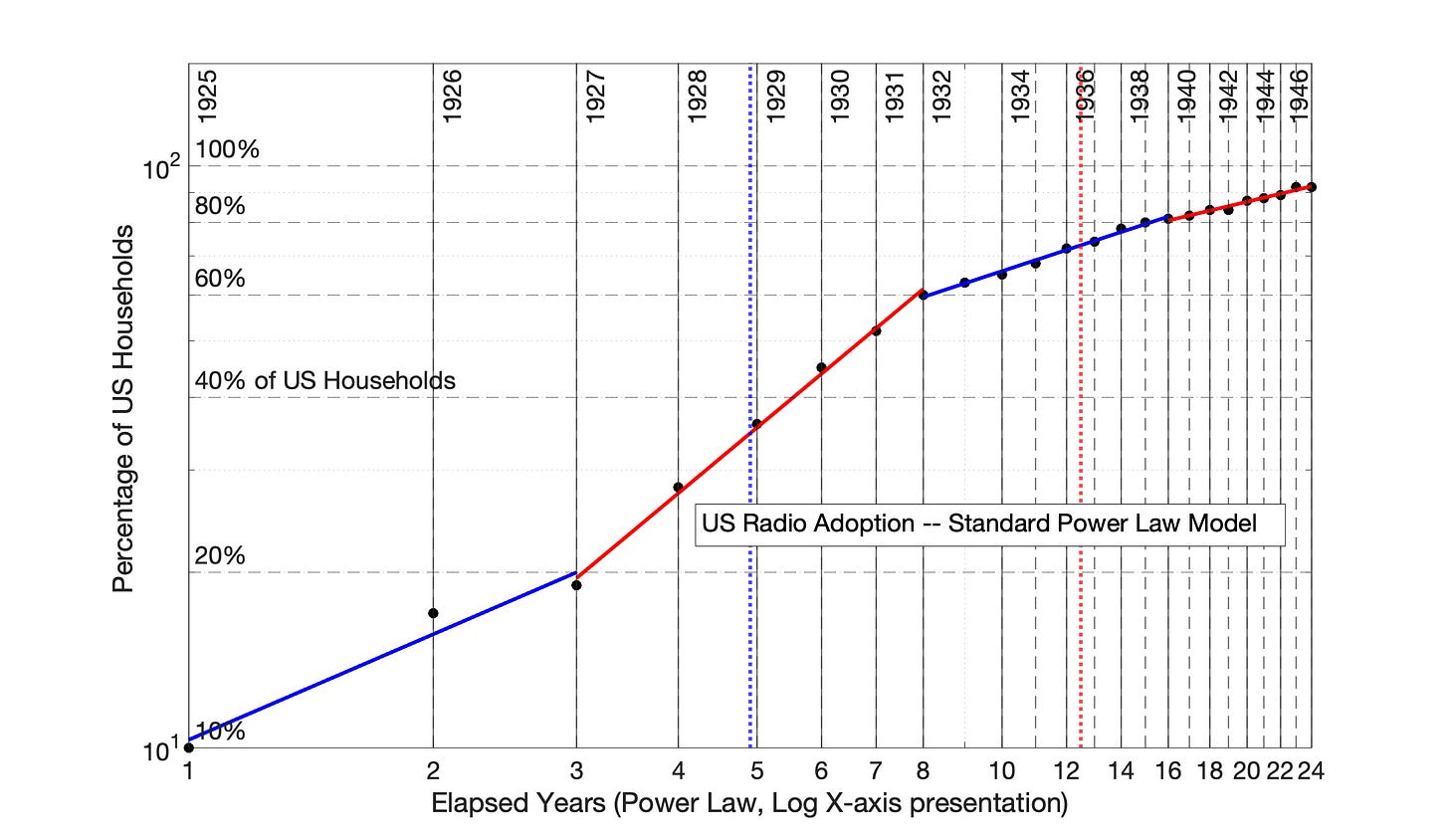
Fig 7.50 US Adoption of Radio, 1925 to 1948: Application of the Square Root of Elapsed Time (SRET) Model. R2 values of linear periods (from left to right) are 0.995, 0.990, 0.991, and 0.976, respectively.
Fig 7.51 US Adoption of Radio, 1925 to 1948: SRET model results from Fig 7.50 are presented as a semilog plot. The identify of the three, linear blue and red periods of Fig 7.50 are shown in this semilog plot of adoption data.
Fig 7.52 US Adoption of Radio, 1925 to 1948: Power Law model with 0 time offset. The Power Law has over-adjusted the initial years of adoption data, creating new data groupings in the first two adoption periods. The R2 values of the four adoption periods, from left to right, are 0.958, 0.997, 0.991 and 0.973.
Fig 7.53 US Adoption of Radio, 1925 to 1948: Power Law model results from Fig 7.52 are presented as a semilog plot. The identify of the 4 adoption periods of Fig 7.52 are shown in this semilog plot of adoption data.
Fig 7.54 US Adoption of Radio, 1925 to 1948: Power Law Model with Data Offset of 3 Years. The convexity of the plotted data in Fig 7.52 is “fixed” by adding 3 years to each time point in the series before application of the Power Law model. This adjustment is displayed at the difference between the x-axis values and adoption years inside the graph. The R2 values of adoption periods, from left to right, are 0.990, 0.992, and 0.974.
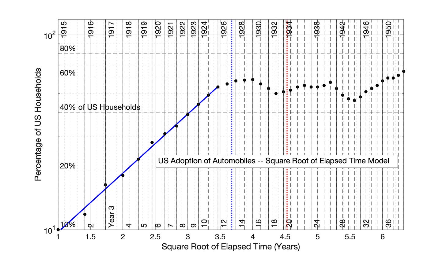
Fig 7.60 US Adoption of the Automobile, 1915 to 1956: Application of the Square Root of Elapsed Time (SRET) Model. R2 value of the initial linear period is 0.996. Adoption was significantly impacted from 1927 to 1944 by the Great Depression and World War II.
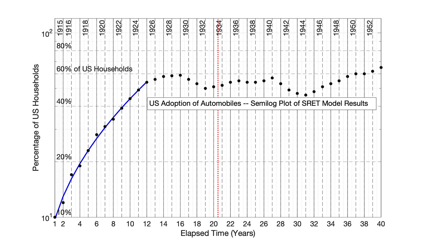
Fig 7.61 U US Adoption of the Automobile, 1915 to 1956: SRET model results from Fig 7.60 are presented as a semilog plot. The identify of the initial, linear blue period of Fig 7.60 is shown in this semilog plot of adoption data.
Fig 7.62 US Adoption of the Automobile, 1915 to 1956: Power Law model with 0 time offset. The Power Law has over-adjusted the initial years of adoption data, creating new data groupings.. The R2 values of the two adoption periods, from left to right, are 0.940 and 0.9995.
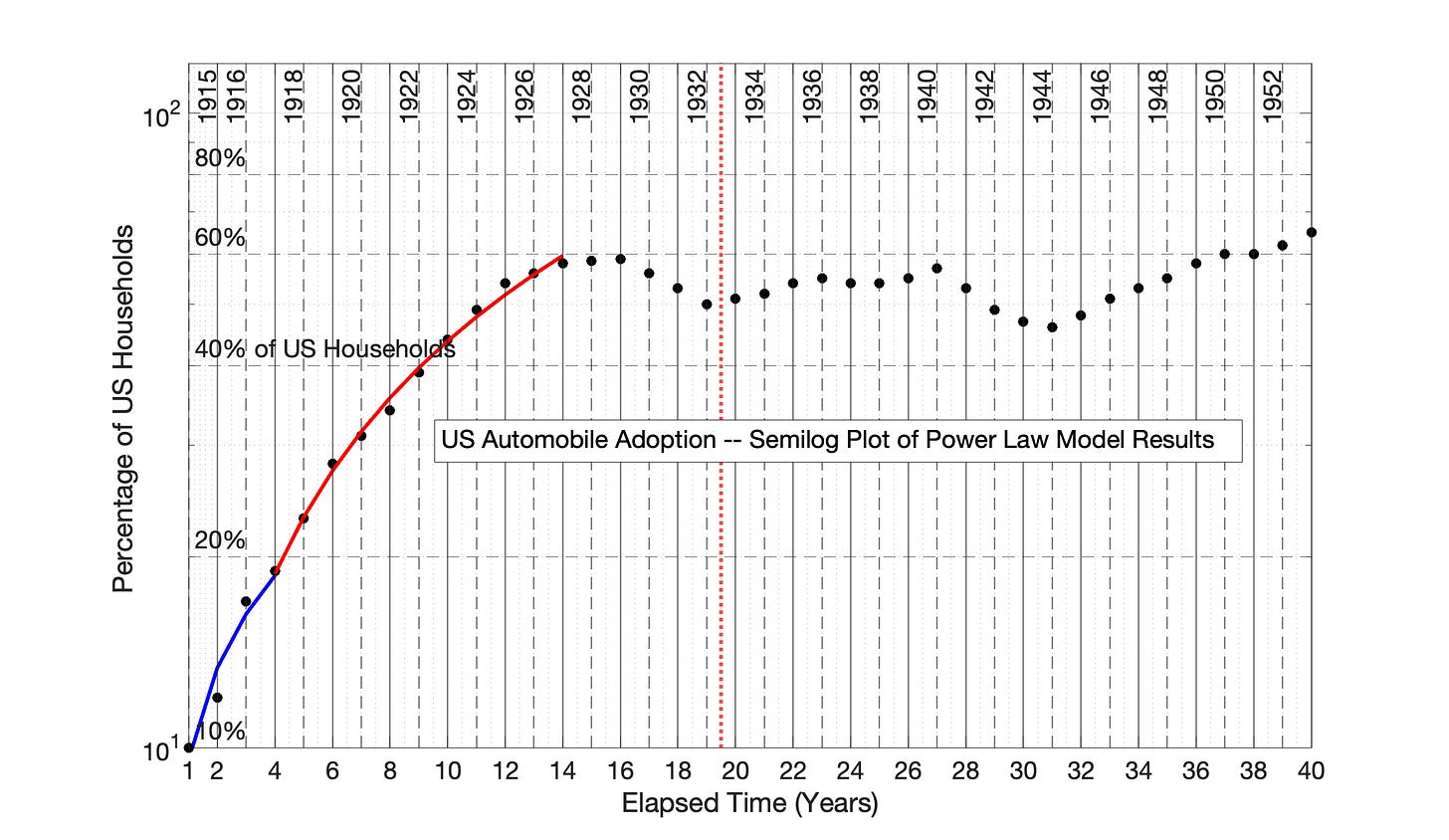
Fig 7.63 US Adoption of the Automobile, 1915 to 1956: Power Law model results from Fig 7.32 are presented as a semilog plot. The identify of the 2 adoption periods of Fig 7.22 are shown in this semilog plot of adoption data.
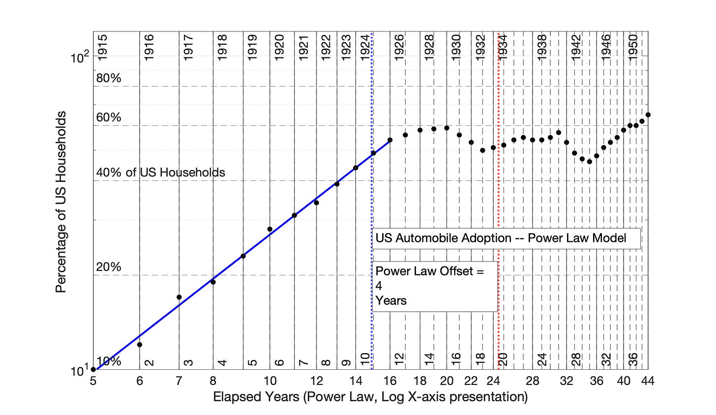
Fig 7.64 US Adoption of the Automobile, 1915 to 1956: Power Law Model with Data Offset of 4 Years. The convexity of the plotted data in Fig 7.62 is “fixed” by adding 4 years to each time point in the series before application of the Power Law model. This adjustment is displayed at the difference between the x-axis values and adoption years inside the graph. The R2 values of the initial adoption period is 0.996.


