Chapter 6. Modeling technology adoptions of the 20th and 21st century: Part 1. When the Power Law Model Succeeds
The Power Law model and the Square Root of Elapsed Time (SRET) model are applied to seven technology adoptions. The two models are equally effective in identifying unique adoptions periods.
6.1 Overview
A new model was developed in Substack Chapters 3, 4 and 5 to model growth of Bitcoin network value (i.e., market cap) and size. This “Square Root of Elapsed Time (SRET) model identifies a significant downturn in the trajectory of Bitcoin market cap and network size growth rate in 2018. This result is at odds with the popular version of the Bitcoin Power Law model, whose advocates assert that Bitcoin growth has seen no trend change since 2009.
The purpose of Chapters 6 through 9 is to gain a thorough understanding of the Power Law and SRET model approaches, to understand the apparent contradiction between these models.
Substack Chapters 6 and 7 begin the comparison of the Power Law and SRET models through examination of 14 prominent technology adoptions of the 20th and 21st centuries — from the US adoption of the automobile and home electrification, to the ongoing worldwide adoption of the internet and cell phones.
These 14 adoptions represent some of the most important technology adoptions in human history, and should provide lessons relevant to the equally important historic adoption of the Bitcoin network in the 21st century.
These technology adoptions were selected at random, but divide naturally into two subgroups. The 7 technology adoptions of Chapter 6 are effectively modeled by both the Power Law and SRET models. The 7 technology adoptions of Chapter 7 are effectively modeled by the SRET model, but NOT by the standard Power Law model. However, the Power Law model can be modified under these circumstances to be effective. Chapters 6 and 7 lay the groundwork for the analysis in Chapters 8 and 9 to resolve the apparent discrepancy between the two modeling approaches for Bitcoin.
The following technology adoptions are modeled by both the Power Law and SRET approaches in Chapter 6
International Internet Adoption, 1990 to 2021
International Cell Phone Adoption, 1980 to 2011
US Social Media Adoption, 2005 to 2019
US Adoption of Home Electricity, 1908 to 1942
US Adoption of Home Microcomputers, 1984 to 2015
US Adoption of Home Air Conditioning, 1957 to 1988
US Adoption of Automobile Radial Tires, 1951 to 1961
Overall Conclusions of Chapters 6:
Technology adoptions share common two common features:
Adoption does not occur in a smooth, “S-shaped” manner. Rather, every technology adoption occurs as a series of discrete “adoption periods”, typically each lasting about 4 to 15 years.
Each adoption period starts with a regime change, typically lasting less than 2 years, to a new adoption rate. Within each adoption period, adoption rate is exponential, but decelerates annually — i.e., exponential, decelerating adoption.
The seven technology adoptions of the 20th and 21 century presented in Chapter 6 are marked by early adoption periods showing rapid adoption but with moderate annual growth deceleration. Both the Power Law model and the SRET model are effective at identifying distinct adoption periods and linearizing the adoption data, but the unadjusted Power Law model is slightly more effective in several cases.
6.2 What are the Power Law and SRET modeling approaches?
The Power Law and the Square Root of Elapsed Time (SRET) modeling approaches are best introduced by describing how technology adoption data is plotted for each model.
In application of the standard Power Law model, network size is plotted in “log” format on the y-axis, and elapsed time is also plotted in “log” format on the x-axis — a “log-log plot”. A linear relationship observed in such a plot follows the model equation,
Natural log of network size = n times the natural log of elapsed time + d
Abbreviated as: ln(N) = n*ln(elapsed time) + d,
Where “ln” is the symbol for natural log, * is the multiplication symbol, and N is the symbol for network size
The constants n and d are the slope and intercept, respectively.
In application of the standard Power Law model, network size is plotted in “log” ln(N)
Note: In subsequent chapters, the Power Law will be presented in its slightly more complex form:
ln(N) = n*ln(elapsed time + time offset) + d
where the time constant is a number greater-than-equal to 0 that must be optimized for each technology adoption.
In Chapter 6, the time offset will be 0 in each case, and the ln(N) equation reduces to the simplified version.
In the SRET model, network size is plotted in “log” format on the y-axis, and elapsed time is plotted as the square root of elapsed time on the x-axis. A linear relationship observed in such a plot follows the model equation,
Natural log of network size = m times (square root of elapsed time) + b
Abbreviated as ln(N) = m*sqrt(elapsed time) + b,
Where “sqrt” is symbol for square root
The constants m and b are the slope and y-intercept, respectively.
6.3 Application of the Power Law and SRET Models: International Adoption of the Internet
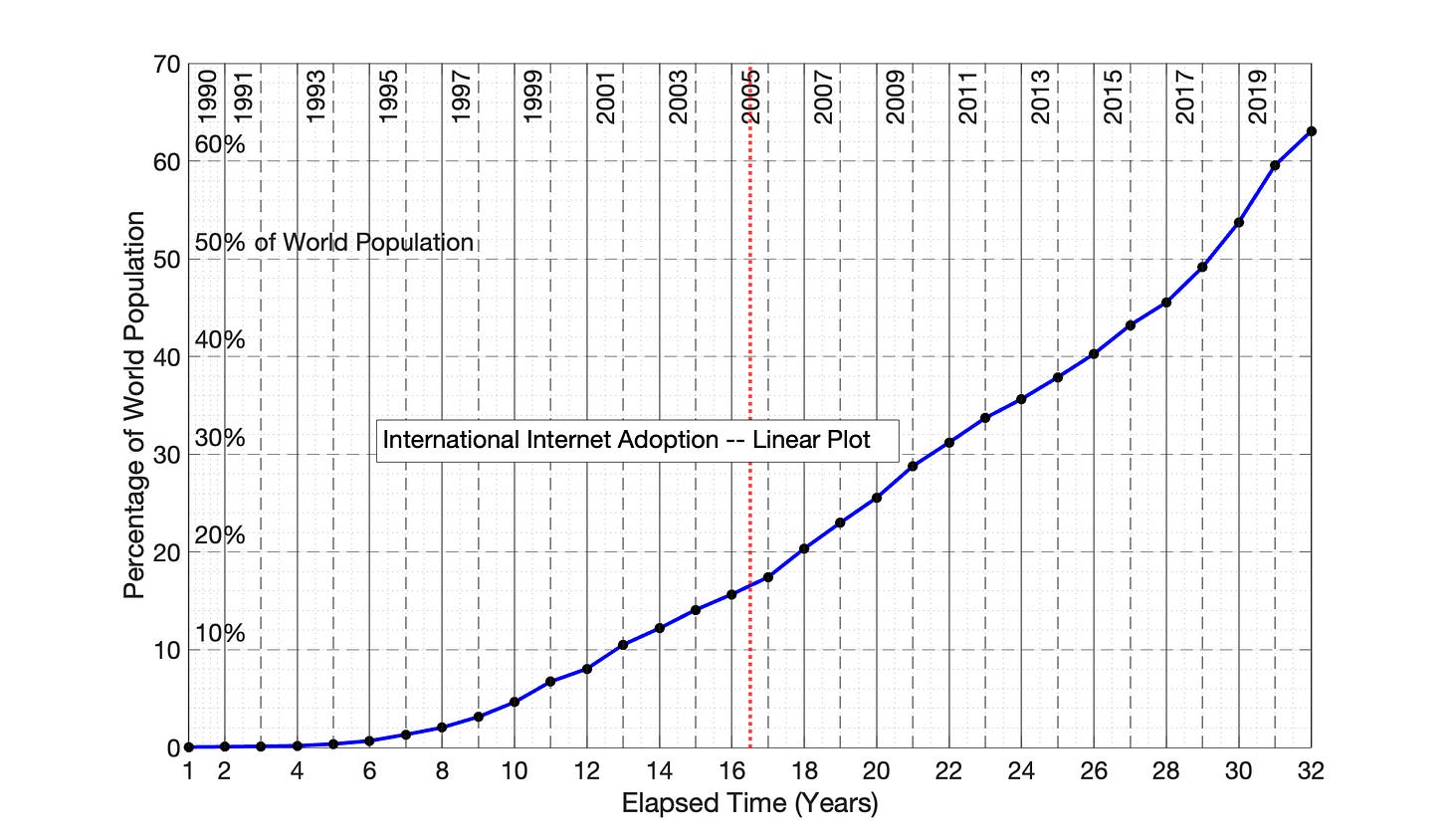
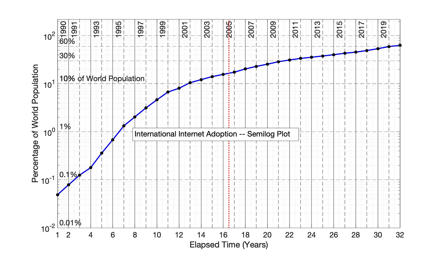
The first technology adoption example is the ongoing international adoption of the internet. In Fig 6.1, data is presented for internet adoption as a function of elapsed time. In Fig 6.2, this data is plotted in a semilog format which more fully captures the full adoption range on the y-axis, from about 0.05% of the world population in 1990 to approximately 60% in 2021.
Important note: The general shape of the semilog plot of Fig 6.2 is typical of ALL of the 16 technology adoptions observed in these Substack Chapters. The network is growing rapidly with time, but the annual rate of increase in network size is decreasing with each subsequent year —decelerating, exponential growth.
Fig 6.1. Diffusion of worldwide internet access, 1990 to 2017: Linear plot of network size, N, vs. elapsed time. Network size, N, is represented as percentage of the world population who had used the internet at least once every 3 months.
Fig 6.2 Diffusion of worldwide internet access, 1990 to 2017: Semilog plot of network size, N, vs. elapsed time. Network size, N, is represented as percentage of the world population who had used the internet at least once every 3 months. This plot demonstrates the rapid, but decelerating growth typical of technology adoptions. The vertical, dotted red line is the temporal and visual midpoint of the graph.
The same data from Figures 6.1 and 6.2 is plotted in the Power Law format in Fig 6.3.
The worldwide adoption of the internet as viewed in Fig 6.3 DOES NOT occur as a smooth, S-shaped adoption curve. Rather, adoption occurs in three distinct “adoption periods,” represented by blue and red straight lines through the data points.
Fig 6.3 provides a first glimpse of how the Power Law model converts the curvature of the semilog plot (Fig 6.2) into distinct linear periods. Both Figures 6.2 and 6.3 have the same Y-axis. The Power Law model creates a mathematical “distortion" of the X-axis. This distortion of the X-axis by the Power Law model results in a differentiated, rightward shift of each of the data points except the first and last, resulting in a linear positioning of the data in Fig 6.3. (A detailed example of this shift is presented in Chapter 7, Section 7.2).
The single, blue and red, vertical, dotted lines in Fig 6.3 represent a means to assess the degree of time expansion/compression by either the Power Law or SRET models. The vertical dotted red line represents the mid-point in elapsed time represented in the graph — the “temporal midpoint”. For example, the elapsed time of Fig 6.3 is 31 years, from 1990 to 2021. There are 15.5 years of adoption data on either side of the red, vertical dotted line.
The vertical blue line represents the “visual mid-point” of the data in Fig 6.3 — the horizontal halfway point of the data presented in the graph — that is, as measured by a ruler. The distance between the vertical, red and blue, dotted lines is a measure of the degree of X-axis time distortion created by the Power Law or SRET model in a particular figure. Another measure of the intensity of time distortion is the difference in width between years on the left and right sides of the graph. Again, the more intense the time distortion, the farther individual points are being shifted to the right in the plot.
Fig 6.3 Worldwide internet access adoption, 1990 to 2021: Power Law model (0 time offset). Network size, N, is measured as the percentage of the world population who have had internet access at least once in three months. The linear blue and red periods can be individually represented by the equation Ln(N) = n*(natural log of elapsed time) + d. The R2 values for the 3 adoption periods (from left to right) are 0.979, 0.998 and 0.997.
The Power Law model equations for the 3 adoption periods in Fig 6.3 are:
Years 1-4, “blue” period: ln(N) = 0.928*(ln of elapsed time) - 3.077
Years 4-13, “red” period: ln(N) = 3.541*(ln of elapsed time) - 6.661
Years 13-32, “blue” period: ln(N) = 1.949*(ln of elapsed time) - 2.631
The purpose of presenting these equations is to remind the reader that solid red and blue lines in Fig 6.3 represent mathematical equations of the “Power Law” type.
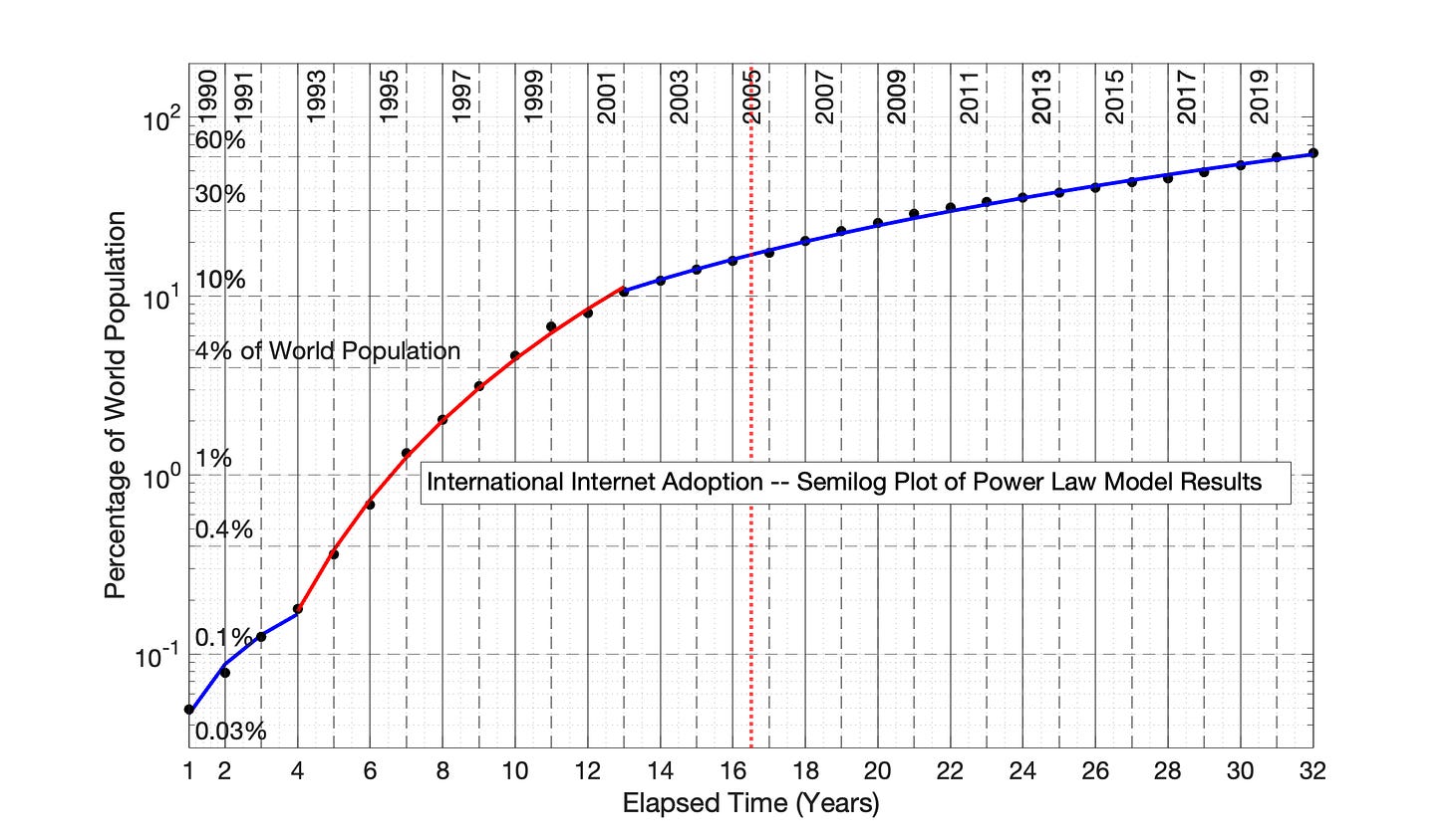
In Fig 6.4, these 3 linear equations are plotted with the original adoption data on a semilog graph — i.e., no time distortion. Fig 6.4 demonstrates:
The excellent fit of the Power Law model to the original data.
The rapid but decelerating growth in each of the 3 adoption periods.
The dotted red line in this figure is a reminder that the temporal midpoint and visual midpoint are the same when results are presented as a semilog plot as a function of time. This convention is repeated in all of the semilog graphs of this Chapter.
Fig 6.4 Worldwide internet adoption, 1990 to 2021: Semilog plot of power law results The power law model fits from Fig 6.3 are presented in semilog format.
The Square Root of Elapsed Time (SRET) model is applied in Fig 6.5. Observations from this figure:
Like the Power Law model, the SRET model distorts the X-axis, expanding early time periods and compressing later time periods to achieve data linearization. However, the amount of time distortion is much less intense than the Power Law model (compare Fig 6.5 to Fig 6.3). This is evident in the relative width of early and late time periods, and also evident in the relative positions of the blue and red, vertical, dotted lines.
The SRET model (Fig 6.5) is effective in identifying the same 3 adoption periods, like the Power Law Model (Fig 6.3).
However, the fit of the adoption data to the SRET model (Fig 6.5) during the 2nd, “red” adoption period is not as good as the Power Law model fit. This is evident visually, and in comparison of the R2 values for 2nd, red adoption period in Fig 6.3 and 6.5. There are some adoption periods for some specific technology adoptions where the more intense time distortion of the Power Law model is appropriate.
Fig 6.5 Worldwide internet access adoption, 1990 to 2021: Square Root of Elapsed Time model. Network size, N, is measured as the percentage of the world population who have had internet access at least once in three months. The linear blue and red periods can be individually represented by the equation Ln(N) = m*(square root of elapsed time) + b. The R2 values for the 3 adoption periods (from left to right) are 0.997, 0.990 and 0.991.
The Square Root of Elapsed Time (SRET) model equations for the 3 adoption periods in Fig 6.5 are:
Years 1-4, “blue” period: ln(N) = 1.309*(sqrt of elapsed time) - 4.359
Years 4-13, “red” period: ln(N) = 2.564*(sqrt of elapsed time) - 6.671
Years 13-32, “blue” period: ln(N) = 0.846*(sort of elapsed time) - 0.608
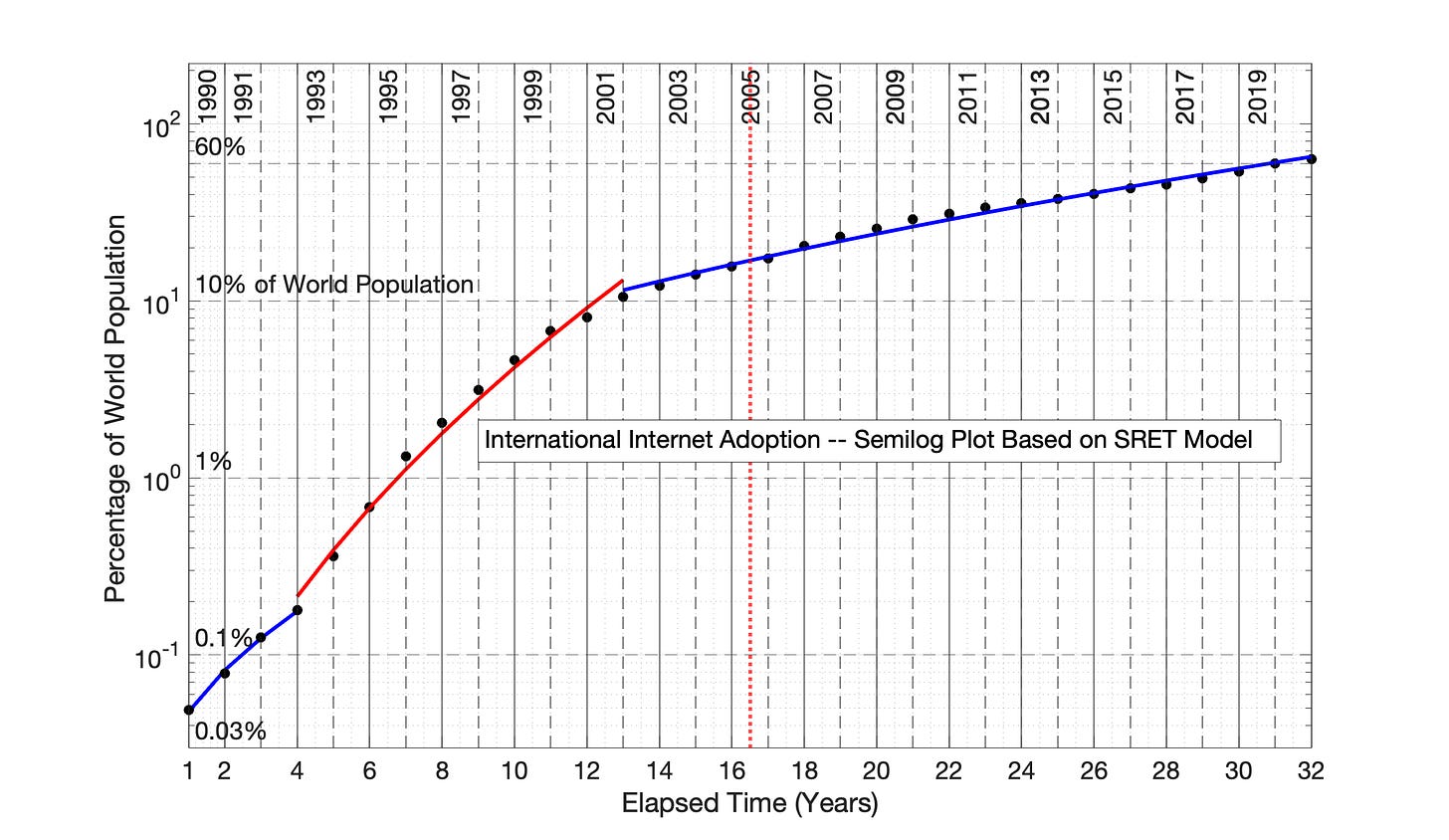
In Fig 6.6, these 3 linear equations determined from Fig 6.5 are plotted with the original adoption data on a semilog graph. The deficiency of the SRET model is matching the sharp data curvature in Period 2 is evident. As stated previously, the Power Model is more effective in modeling periods with exponential but strongly decelerating annual growth rate.
Fig 6.6 Worldwide internet access adoption, 1990 to 2021: Semilog plot of SRET model results The SRET model fits from Fig 6.5 are presented in semilog format.
The remaining six technology adoptions presented in Chapter 6 share common features with the figures presented above.
Each technology adoption is marked by distinct adoption periods
The Power Law and SRET models both identify the same periods
In several cases, the Power Law is marginally better at linearizing the data for specific, early adoption periods.
6.4 Quantifying Rapid but Decelerating Growth
Table 6.1 presents the observed values of percentage international adoption (column 3), plus the predicted values from the 2 models (columns 5 and 7). The annual percentage increase in observed adoption is presented in column 4, while the percentage increases from the Power Law and SRET models are presented in columns 6 and 8, respectively.
The percentage annual increases in adoption (columns 4, 6 and 8) are color-coded to match the 1st red period and 2nd blue period from Figures 6.3 and 6.5.
A first observation in Table 6.1 is that the two models effectively modeled network size during each period. A second observation is that the “regime change” from one period to another is marked by a relatively sharp change in adoption rate. A third observation is that each period is marked by a decelerating annual increase in adoption rate.
Differences in the predictions of the two models are related to the respective fits of model data. From visual observation of Figures 6.3 and 6.5 and the R2 values, the Power Law model is more effective in linearizing the second, “red” adoption period.
Table 6.1 Worldwide adoption of the internet, 1990 to 2014: Network size data and calculations. Percentage of world population who used the internet once in the past 3 months is the proxy for network size. Predicted network size values from the Power Law model are presented for comparison to the observed values. Annual increases are color-coded to match the red and second blue periods lines in Figures 6.3/6.4 and 6.5/6.6.
6.5 The Power Law and Square Root of Elapsed Time modeling approaches work for a variety of other technology adoptions.
Six additional technology adoptions of the 20th and 21st centuries are evaluated by the Power Law and SRET models, with figures presented in the Appendix.
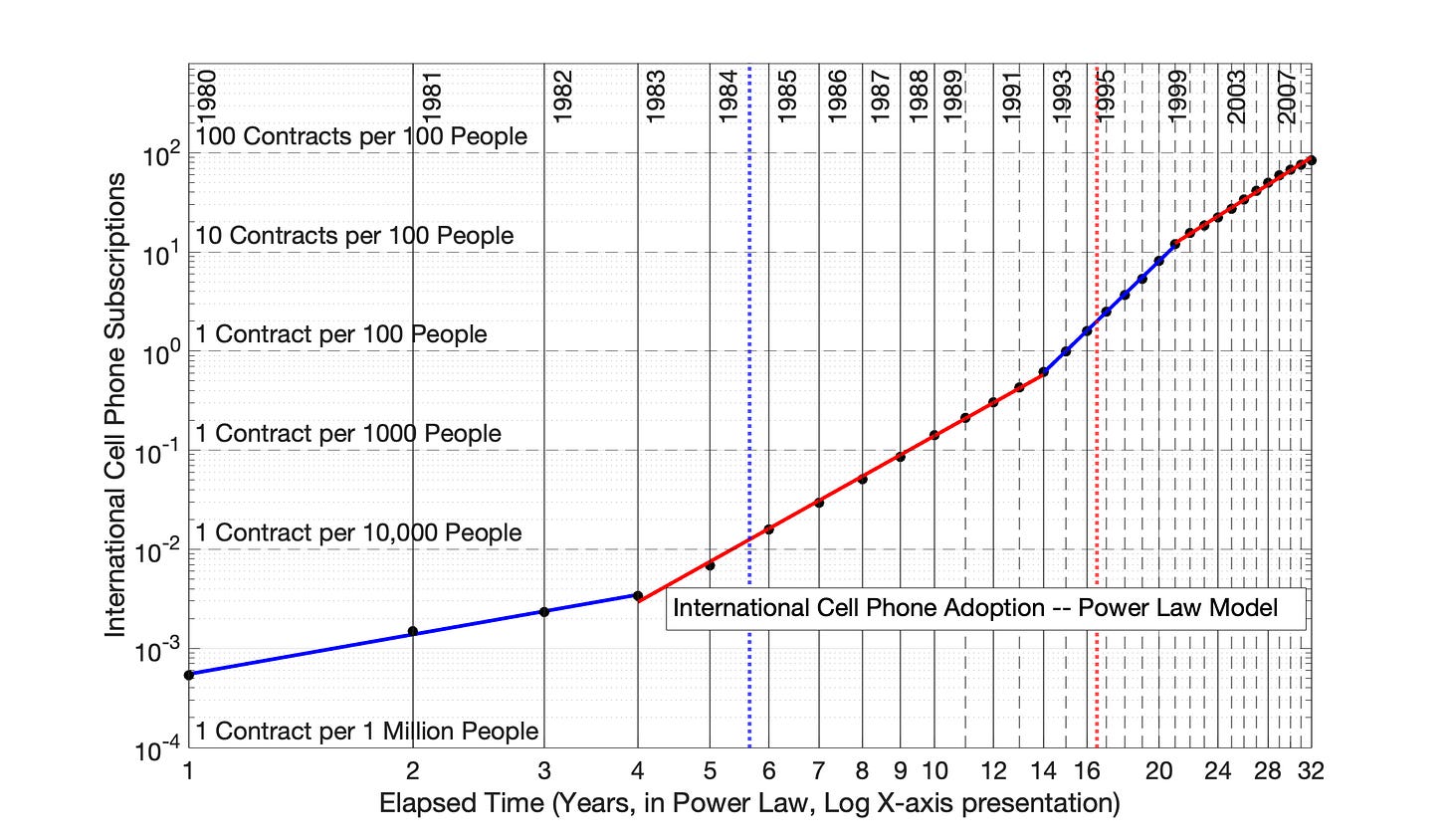
Fig 6.7 International Cell Phone Adoption, 1980 to 2011: Power Law model (0 time offset)
Fig 6.8 International Cell Phone Adoption, 1980 to 2011: Power Law model results presented in semilog format
Fig 6.9 International Cell Phone Adoption, 1980 to 2011: Square Root of Elapsed Time model
Fig 6.10 US Social Media Adoption, 2005 to 2019: Power Law model (0 time offset)
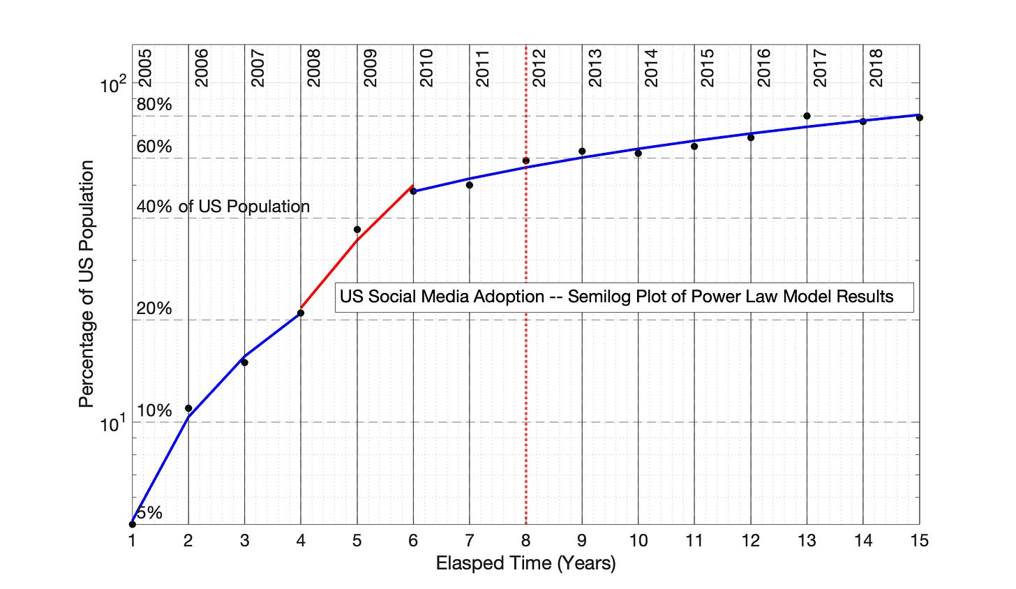
Fig 6.11 US Social Media Adoption, 2005 to 2019: Power Law model results presented in semilog format
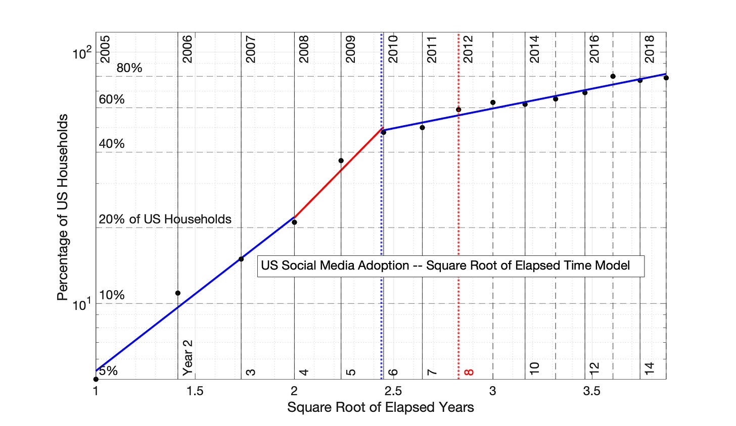
Fig 6.12 US Social Media Adoption, 2005 to 2019: Square Root of Elapsed Time (SRET) model
Fig 6.13 US Adoption of Home Electricity, 1908 to 1942: Power Law model
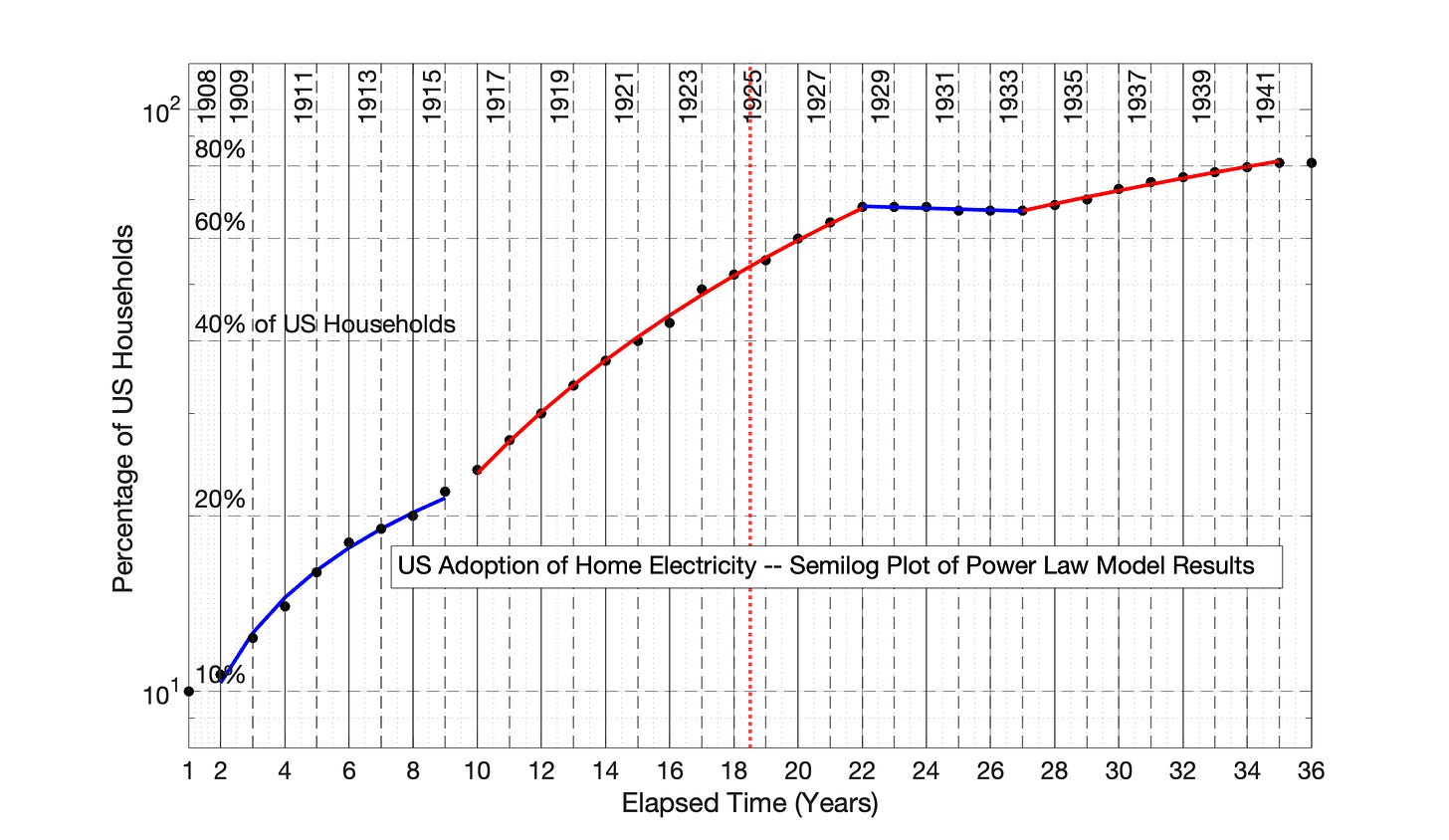
Fig 6.14 US Adoption of Home Electricity, 1908 to 1942: Power Law model results presented in semilog format
Fig 6.15 US Adoption of Home Electricity, 1908 to 1942: Square Root of Elapsed Time (SRET) model
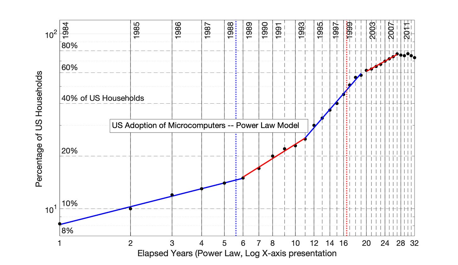
Fig 6.16 US Adoption of Home Microcomputers, 1984 to 2015: Power Law model (0 time offset)
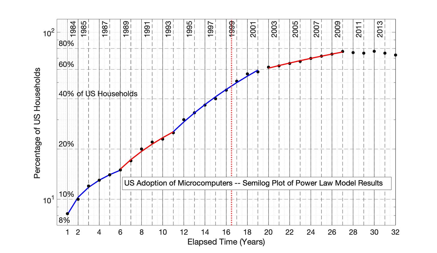
Fig 6.17 US Adoption of Home Microcomputers, 1984 to 2015: Power Law model results presented in semilog format
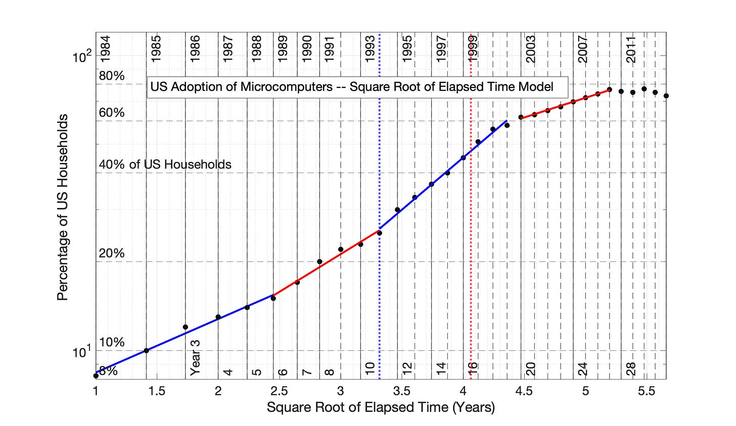
Fig 6.18 US Adoption of Home Microcomputers, 1984 to 2015: Square Root of Elapsed Time (SRET) model
Fig 6.19 US Adoption of Home Air Conditioning, 1957 to 1988: Power Law model (0 time offset)
Fig 6.20 US Adoption of Home Air Conditioning, 1957 to 1988: Power Law model results presented in semilog format
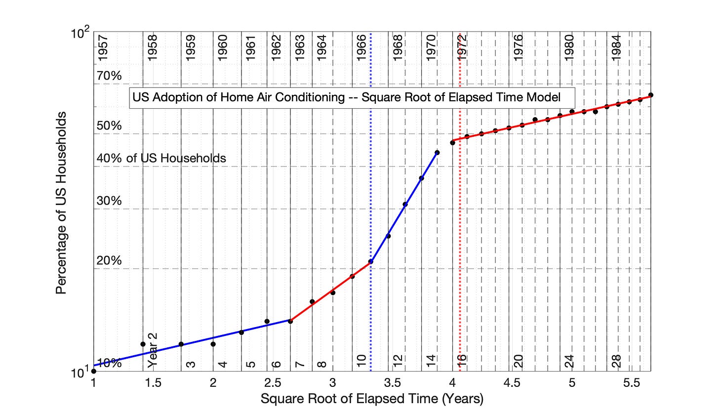
Fig 6.21 US Adoption of Home Air Conditioning, 1957 to 1988: Square Root of Elapsed Time (SRET) model
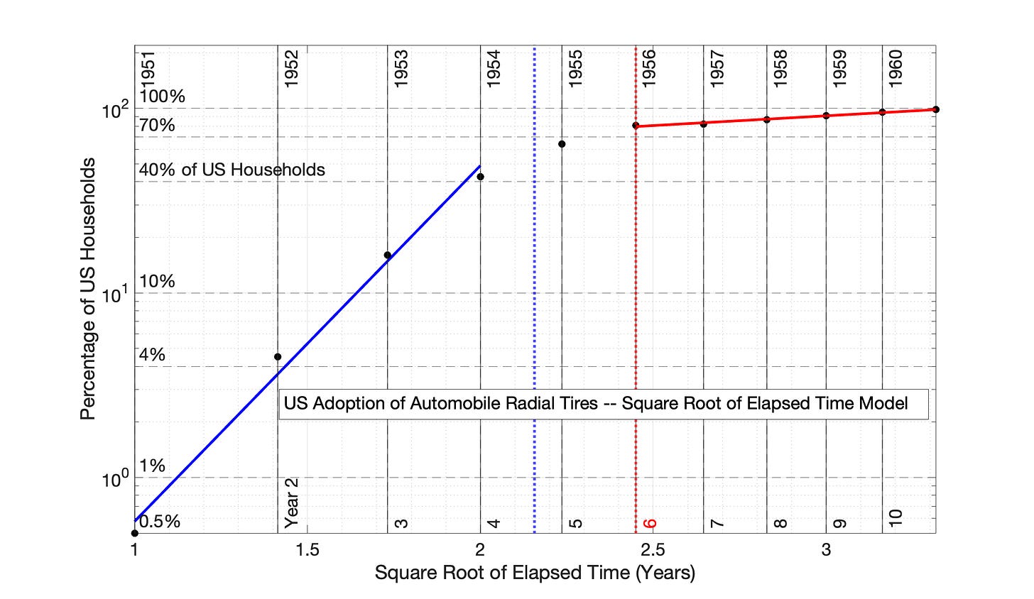
Fig 6.22 US Adoption of Automobile Radial Tires, 1951 to 1961: Power Law model (0 time offset)
Fig 6.23 US Adoption of Automobile Radial Tires, 1951 to 1961: Power Law model results presented in semilog format
Fig 6.24 US Adoption of Automobile Radial Tires, 1951 to 1961: Square Root of Elapsed Time (SRET) model
6.6 Chapter Conclusions
General conclusions are stated at the end of Section 6.1.
The Power Law model is somewhat more effective at linearizing adoption data for periods experiencing rapid growth with moderate to sharp adoption deceleration — as judged by both visual comparison and R2 value. Examples are identified below.
That is, for these technology adoption periods, a greater amount of time distortion was necessary to linearize the data, and the Power Law model provided this higher level of time distortion. The SRET model did not provide enough time distortion to completely linearize the data.
International Internet Adoption, Period 2 (Compare Figures 6.3 and 6.5)
International Cell Phone Adoption, Period 2 (Figures 6.7 and 6.9)
US Social Media Adoption, Period 1 (Figures 6.10 and 6.12)
US Adoption of Microcomputers, Periods 1 and 2 (Figures 6.16 and 6.18)
US Adoption of Automobile Radial Tires, Period 1 (Figures 6.22 and 6.24)
In defense of the SRET model: In every case it was capable of identifying the distinct linear adoption periods, and while linearization was not perfect in the stated cases, the amount of linearization provided by the SRET model was sufficient to obtain reasonable model equations.
A detailed summary of Chapter 6 and 7 results will be presented at the conclusion of Chapter 7.
6.7 Data Sources
The online journal ourworldindata.org provides historical data on the adoption of technologies in the US and worldwide. To access the specific data employed in this manuscript, open ourworldindata.org, then in the search box type:
“Mobile phone subscription” to reach the page allowing download of mobile phone subscriptions per 100 people worldwide.
“Share of the population using the internet” to reach the page allowing download the data for the share of the world population who have used the internet in the last 3 months.
“Share of US households using specific technologies” to reach the page allowing download of this data. (Reference: Hannah Ritchie and Max Roser, 2017, "Technology Adoption". Published online at OurWorldInData.org.)
The data for growth of Facebook network size is from Zhang, X, Liu, J, and Xu, Z. “Tencent and Facebook Data Validate Metcalfe’s Law,” J. Computers Science and Technology, 2: 246-251, 2015, and from Facebook Annual Reports.
6.8 About the Author
The author has a B.S. and PhD. In chemical engineering. His PhD thesis focussed on mathematical modeling, simulation, and implementation of process control. Following his PhD, he was a university professor for 10 years at two US universities, focusing on both research and teaching. At both universities he taught the required chemical engineering course in process modeling and control. He subsequently spent more than 20 years in industrial chemical engineering practice.
6.9 Appendix
Fig 6.7 International Cell Phone Adoption, 1980 to 2011: Power Law model (0 time offset) Cell phone contracts per 100 people worldwide is the measure of network adoption. The vertical, dotted red line represents the temporal midpoint of data presented on the x-axis, while the vertical, dotted blue line represents the visual midpoint of the x-axis data. The R2 values for the 4 adoption periods (from left to right) are 0.996, 0.998, 0.999 and 0.997.
Fig 6.8 International Cell Phone Adoption, 1980 to 2011: Semilog plot of power law results The power law model results from Fig 6.7 are presented in semilog format.
Fig 6.9 International Cell Phone Adoption, 1980 to 2011: Square Root of Elapsed Time (SRET) model Cell phone contracts per 100 people worldwide is the measure of network adoption. The R2 values for the 4 adoption periods (from left to right) are 0.976, 0.996, 0.9996 and 0.994.
Fig 6.10 US Social Media Adoption, 2005 to 2019: Power Law model (0 time offset) Percentage of US Households is the proxy for network size. The R2 values for the 3 adoption periods (from left to right) are 0.995, 0.977, 0.999 and 0.947.
Fig 6.11 US Social Media Adoption, 2005 to 2019: Semilog plot of power law results The power law model fits from Fig 6.10 are presented in semilog format.
Fig 6.12 US Social Media Adoption, 2005 to 2019: Square Root of Elapsed Time (SRET) model. Percentage of US Households is the proxy for network size. The R2 values for the 3 adoption periods (from left to right) are 0.978, 0.967, and 0.941.
Fig 6.13 US Adoption of Home Electrical Power, 1908 to 1942: Power Law model (0 time offset) Percentage of US Households is the proxy for network size. The R2 values for the 4 adoption periods (from left to right) are 0.991, 0.999, 0.770 and 0.982.
Fig 6.14 US Adoption of Home Electrical Power, 1908 to 1942: Semilog plot of power law results The power law model fits from Fig 6.13 are presented in semilog format.
Fig 6.15 US Adoption of Home Electrical Power, 1908 to 1942: Square Root of Elapsed Time (SRET) model. Percentage of US Households is the proxy for network size. The R2 values for the 3 adoption periods (from left to right) are 0.993, 0.978, 0.771 and 0.990.
Fig 6.16 US Adoption of Home Microcomputers, 1984 to 2015: Power Law model (0 time offset) Percentage of US Households is the proxy for network size. The R2 values for the 3 adoption periods (from left to right) are 0.995, 0.984, 0.999 and 0.991.
Fig 6.17 US Adoption of Home Microcomputers, 1984 to 2015: Semilog plot of power law results The power law model fits from Fig 6.16 are presented in semilog format.
Fig 6.18 US Adoption of Home Microcomputers, 1984 to 2015: Square Root of Elapsed Time (SRET) model Percentage of US Households is the proxy for network size. The R2 values for the 3 adoption periods (from left to right) are 0.983, 0.975, 0.993 and 0.994.
Fig 6.19 US Adoption of Home Microcomputers, 1984 to 2015: Semilog plot of power law results The power law model fits from Fig 6.18 are presented in semilog format.
Fig 6.20 US Adoption of Home Air Conditioning, 1957 to 1988: Power Law Model (0 time offset) Percentage of US Households is the proxy for network size. The R2 values for the 3 adoption periods (from left to right) are 0.903, 0.989, 0.998 and 0.990.
Fig 6.21 US Adoption of Home Air Conditioning, 1957 to 1988: Square Root of Elapsed Time (SRET) model Percentage of US Households is the proxy for network size. The R2 values for the 3 adoption periods (from left to right) are 0.893, 0.991, 0.999 and 0.990.
Fig 6.22 US Adoption of Automobile Radial Tires, 1951 to 1961: Power Law model (0 time offset) Percentage of US Households is the proxy for network size. The R2 values for the 3 adoption periods (from left to right) are 0.9998 and 0.968.
Fig 6.23 US Adoption of Automobile Radial Tires, 1951 to 1961: Semilog plot of power law results The power law model fits from Fig 6.22 are presented in semilog format.
Fig 6.24 US Adoption of Automobile Radial Tires, 1951 to 1961: Square Root of Elapsed Time (SRET) model Percentage of US Households is the proxy for network size. The R2 values for the 3 adoption periods (from left to right) are 0.992 and 0.978.


