
Chapter 11. Two New Models Define How Bitcoin Market Cap is Affected by Both the Growth of Network Size and Time
Network Value "Model 1" and "Model 2" are introduced, expressed in both the Square Root of Elapsed Time (SRET) and Power Law model formats.

11.1 Introduction
First-level models explain the relationship of a single output variable (e.g., market cap) to a single input variable (e.g., time). For example,
SRET model: ln(market cap) = m*sqrt(elapsed time) + b
Power Law model: ln(market cap) = n*ln(elapsed time + time offset) + d
Where m, b, n, d , and the time offset are constants determined from data analysis.
ln, sqrt, and * are the symbols for natural logarithm, square root, and multiplication, respectively
First-level SRET and Power Law models were developed in Chapter 8 for the growth of Bitcoin network size. First-level SRET and Power Law models were developed in Chapter 9 for the growth of Bitcoin market cap.
A second-level model explains the interaction of more than 2 factors. In technology adoption, such a model would typically explain the interactions of:
the growth of network value, V (e.g., market capitalization)
the growth of network size, N
elapsed time, t
Robert Metcalfe famously developed a “network value” model describing the interrelationship of these three factors (1). Metcalfe’s model included two equations:
A proposed relationship between V and N — specifically, V = c*N2, where c is a constant. This equation has been termed “Metcalfe’s Law.”
And, a second equation describing the growth of N with time.
The first purpose of this chapter is to develop two new network value models, with the Bitcoin network as a case study. The first model (“Model 1”) expresses the relationship between V, N and time in two equations, and the second model (“Model 2”) captures this relationship in a single equation of V as a function of N and time. Model 1 provides new insight into the magnitude of the change that occurred in the Bitcoin network in 2018. Model 2 is potentially a powerful new tool for evaluating the Bitcoin network, particularly during periods of network transition — i.e., like the 2018 transition.
The second purpose of this chapter is to show that the two models can be expressed in two different equation formats, the Square Root of Elapsed Time (SRET) model and the Power Law model.
The SRET and Power Law model equations are developed in Substack Chapters 6 through 10. A synopsis of each chapter and a link to each are presented in the Appendix 2 of this chapter.
Let me mention this just once in the main body of this Chapter. One of the most consequential events in Bitcoin history was the transition that occurred in 2018. The blistering Bitcoin network growth trajectory of 2012-2018 declined to a more sustainable, rapid growth trajectory after 2018. The growth trajectory of network participants (i.e., network size) also declined in 2018.
(Note: If the growth trajectory of 2012 to 2018 had been maintained, the Bitcoin network would have had a value of approximately $300 to $600 Trillion by 2034, much more than all of the equities in the world (see Substack Chapter 10). This would correspond to a price of more than $10 million per Bitcoin. The author does not doubt that Bitcoin will eventually reach this goal — just not by 2034)
Both the SRET model and the Power Law Model employed in these Substack Chapters provide consistent documentation of the 2018 adoption rate shift.
The version of the Power Law Model employed in these Substack analyses is different from the version employed by Giovanni Santostasi in his Twitter version of the Power Law.
Chapters 6 through 10 of this Substack document the case in favor of the version of the Power Law employed in this Substack chapter, which includes a time offset factor with a value of 2000 days (5 years). Synopses and links to Substack Chapters 6 through 10 are presented in Appendix 2 of this Chapter.
11.2 The First Network Value Model, Expressed as SRET Model Equations (“Model 1A”)
Model 1 is composed of two equations, one describing the growth of network size, N, with time, and a second equation describing the growth of network value, V, with time. For Bitcoin, V, would typically represent Bitcoin market cap (number of Bitcoin in circulation times price). In Substack Chapter 8, it was shown that the count of Bitcoin-containing addresses has been a suitable metric for Bitcoin network size — i.e., Addresses with >0 Bitcoin.
Note: For the models being explored in these Substack chapters, a metric for Bitcoin network size does NOT need to be an absolute measure of Bitcoin network size. The metric just needs to be consistently proportional to network size.
Model 1 is expressed in two forms in this Chapter. Model 1A is the version expressed in terms of the SRET model format. Model 1B is the version expressed in terms of the Power Law format.
The two equations of Model 1A are:
Eq 11.1: ln(N) = m1*sqrt(elapsed time) + b1
Eq 11.2: ln(V) = m2*sqrt(elapsed time) + b2
Where N and V are the symbols for network size and network value, respectively
ln and sqrt are the symbols for natural logarithm and square root
m1, m2, b1 and b2 are constants
These two equations are of the form y = m*x + b, the equation of a straight line, with m as the slope and b as the y-intercept.
The SRET model equation ln(N) = m*sqrt(elapsed time) + b was shown in Chapters 6 and 7 to be effective in modeling individual adoption periods for 14 historic technology adoptions of the 20th and 21st century — e.g., the international adoption of the internet in the 21st century.
In Chapter 8, this equation is effective in modeling Bitcoin-containing address count as a metric for Bitcoin network size — the Period 1 and 2 blue lines in Fig 11.1.
The model equation ln(V) = m*sqrt(elapsed time) + b is effective in modeling Bitcoin market cap as the metric for network value — the Period 1 and Period 2 blue lines of Fig 11.2. The market cap data BETWEEN historic Bitcoin “bull runs” was shown to be suitable for this modeling (Chapter 9). The market cap data during “bull” runs was shown in Chapter 9 to be inappropriate for a network value model — these are periods in which network value has disconnected from network size.
The two equations described above are individually valuable in describing the first-level relationships of network size and network value to time for a particular adoption period.
As a pair of equations, these two equations are a network value model. Together, they explain the relationship between network size and network value in a particular adoption period (provided that both equations are linear during that adoption period). That is, because N and V are both related to time by these two, Model 1A equations, it is possible to derive the relationship between V and N.
In Appendix 1, Section A1.1, it is shown that the relationship between V and N is:
V = c*Nx, where c and x are constants
The constants c and x are computed from the model equation coefficients, m1, m2, b1 and b2:
x = m2/m1
ln(c) = b2 - b1*x or c = e(b2 - b1*x)
For example, if m2/m1 = 2, the equation becomes Metcalfe’s Law, V = c*N2.
The SRET model relationships for Bitcoin network size and network value were determined in Chapters 8 and 9:
Period 1, before 2018:
Chapter 8: ln(Addresses) = 0.1230*(sqrt of elapsed time) + 10.22
Chapter 9: ln(Market Cap) = 0.2428*sqrt(elapsed time) + 11.61
Period 2, after 2018:
Chapter 8: ln(Addresses) = 0.05262*(sqrt of elapsed time) + 14.06
Chapter 9: ln(Market Cap) = 0.1420*sqrt(elapsed time) +17.29
In the equations of these Substack Chapters, market cap is expressed in US dollars and elapsed time is expressed in days after 17Jul2010, the first day in the Glassnode time series for Bitcoin price and market cap.
For Period 1: x2/x1 = 0.2428/0.1230 = 1.97 while c = 1.89 x 10⁴
For Period 2: x2/x1 = 0.1420/0.05262 = 2.70, while c = 1.08 x 10⁹
In summary, the relationships of Bitcoin market cap to Bitcoin-containing addresses are:
2012 to 2018: V = c*N1.97 , with c = 1.89 x 10⁴, and
2019 to 01Jul2024: V = c*N2.70 , with c = 1.08 x 10⁹.
For the period from 2012 to 2018, this result is consistent with the previous observation that the Bitcoin network followed Metcalfe’s Law, V = c*N2 (references 2-5).
This results of this section emphasize the considerable change that occurred in the Bitcoin network after 2018. The relationships of both N and V to elapsed time changed (as shown in Figures 11.1 and 11.2), and the relationship of N to V also changed.
This result shows the strength and versatility of Model 1. It is NOT necessary for us to assume that a particular technology diffusion is governed by Metcalfe’s Law, V = c*N2. After we solve for the Model 1A slopes and intercepts (m1, m2, b1, b2) for a particular adoption period, the coefficients m1, m2, b1 and b2 allow calculation of the relationship between N and V.

Fig 11.1 SRET Model Plot for Bitcoin-Containing Addresses (i.e., the metric for network size) This figure was presented previously as Fig 8.3 (i.e., the third figure in Substack Chapter 8). The blue lines represent the least-squares, best-fitting, SRET model straight lines for Periods 1 (01Jan2012 to 01Sep2018) and Period 2 (01Sep2018 to 01Jul2024. The dashed black line Is the linear extension of the Period 1 model fit, to visualize the extent of the adoption downshift that occurred in Period 2. The data points marked in red were included in the model fit. Details of determining the red data points and generating the linear model fit are presented in the Appendix 1, Part 2 (Section 11.11.2). The R2 of the model fits are 0.999 and 0.994, for Periods 1 and 2, respectively.

Fig 11.2 SRET Model Plot for Bitcoin Market Cap (i.e., the metric for network value). This figure was presented previously as Fig 9.1. The blue lines represent the least-squares, best-fitting, SRET model straight lines for Periods 1 (01Jan2012 to 01Jan2019) and Period 2 (01Jan2019 to 01Jul2024). The dashed black line Is the linear extension of the Period 1 model fit, to visualize the extent of the adoption downshift that occurred in Period 2. The data points marked in red were included in the model fit. Details of determining the red data points and generating the linear model fit are presented in the Appendix 1, Part 2 (Section 11.11.2). The R2 of the model fits are 0.995 and 0.933, for Periods 1 and 2, respectively.
11.3 The First Network Value Model, Expressed as Power Law Model Equations (“Model 1B”)
The model equation ln(N) = n*ln(elapsed time + time offset) + d was shown in Chapters 6 and 7 to be effective in modeling individual adoption periods for 14 historic technology adoptions of the 20th and 21st century. The growth of Bitcoin-containing address count is effectively modeled by this equation (Chapter 8). This equation defines the blue lines for Periods 1 and 2 in Fig 11.3.
The model equation ln(V) = n*ln(elapsed time + time offset) + d effectively models Bitcoin market cap in the period between “bull runs” (Chapter 9). These equations were the blue lines for Periods 1 and 2 in Fig 11.4.
The time offset of 2000 days is optimal for modeling the growth of Bitcoin network size and network value (Chapters 8, 9, and 10).
The two equations of Model 1B, describing a particular adoption period are:
Eq 11.3: ln(N) = n1*ln(elapsed time + time offset) + d1
Eq 11.4: ln(V) = n2*ln(elapsed time + time offset) + d2
where n1, n2, d1, d2 and the time offset are constants
Period 1, before 2018:
Chapter 8: ln(Addresses) = 5.725*ln(elapsed time+ 2000) - 31.75
Chapter 9: ln(Market Cap) = 11.24*ln(elapsed time +2000) - 70.76
Period 2, after 2018:
Chapter 8: ln(Addresses) = 2.502*ln(elapsed time+ 2000) - 4.379
Chapter 9: ln(Market Cap) = 6.747*ln(elapsed time +2000) - 32.41
These equations permit the calculation of the relationship of N and V by the equation V = c*Nx (as shown in Appendix 1, Section A1.1 and in Section 11.2)
For Period 1: x2/x1 = 11.24/5.725 = 1.96, where c = 2.19 x10⁴
For Period 2: x2/x1 = 0.1433/0.05262 = 2.70, where c = 1.12 x 10⁹
The results from the Power Law model (with 2000 day time offset), are very similar to the SRET model from the previous section:
From Model 1B (based on the Power Law equation format, with 2000 day time offset), the relationships are:
2012 to 2018: V = c*N1.96 , with c = 2.19 x 10⁴, and
2019 to 01Jul2024: V = c*N2.70 , with c = 1.12 x 10⁹.
These are very similar to the relationships defined in the previous section from Model 1A (based on the SRET equation format):
2012 to 2018: V = c*N1.97 during 2012 to 2018 with c = 1.89 x 10⁴, and
2019 to 01Jul2024: V = c*N2.70 , with c = 1.08 x 10⁹.
In summary, both model approaches are consistent with the relationship V = c*N2 (i.e., Metcalfe’s Law) during 2012 to 2018 and V = c*N2.7 after 2019. Both models emphasize the significant shift that occurred in the Bitcoin network after 2018.

Fig 11.3 Power Law Model Plot (with 2000 day time offset) for Bitcoin-Containing Addresses This figure was presented previously as Fig 8.9. The blue lines represent the least-squares, best-fitting, Power Law model straight lines for Periods 1 (01Jan2012 to 01Sep2018) and Period 2 (01Sep2018 to 01Jul2024. The dashed black line Is the linear extension of the Period 1 model fit, to visualize the extent of the adoption downshift that occurred in Period 2. The data points marked in red were included in the model fit. The magenta arrow points at the smooth transition between the Period 1 and 2 data achieved with a time offset of 2000 days. Details of determining the red data points and generating the linear model fit are described in the Appendix 1, Part 2 (Section 11.11.2). The R2 of the model fits are 0.999 and 0.994, for Periods 1 and 2, respectively.

Fig 11.4 Power Law Model Plot (with 2000 day time offset) for Bitcoin Market Cap This figure was presented previously as Fig 9.9. The blue lines represent the least-squares, best-fitting, Power Law model straight lines for Periods 1 (01Jan2012 to 01Sep2018) and Period 2 (01Sep2018 to 01Jul2024. The dashed black line Is the linear extension of the Period 1 model fit, to visualize the extent of the adoption downshift that occurred in Period 2. The data points marked in red were included in the model fit. The magenta arrow points at the smooth transition between the Period 1 and 2 data achieved with a time offset of 2000 days. Details of determining the red data points and generating the linear model fit are described in the Appendix 1, Part 2 (Section 11.11.2). The R2 of the model fits are 0.994 and 0.933, for Periods 1 and 2, respectively.
11.4 Deriving the 2nd Network Value Model, Expressed in SRET Equation Format (“Model 2A”)
Network Value Model 2 is a single-equation describing the relationship of V to N and elapsed time. Model 2 can be presented in the SRET model format (Model 2A) or the Power Law model format (Model 2B).
From Section 11.2, Model 1A for Bitcoin is the combination of the two equations
Eq 11.1: ln(N) = m1*sqrt(elapsed time) + b1
Eq 11.2: ln(V) = m2*sqrt(elapsed time) + b2
Model 2A is derived as follows. First, subtract Eq 11.1 from Eq 11.2:
ln(V) - ln(N) = (m2-m1)*sqrt(elapsed time) + (b2 - b1)
An established relationship for logarithmic functions is ln(y) - ln(x) = ln(y/x). Therefore, the equation just above can be simplified to:
Eq 11.5: ln(V/N) = m3*sqrt(elapsed time) + b3
This equation defines Network Value Model 2A.
Where m3 and b3 are the slope and intercept of a plot of ln(V/N) vs the square root of elapsed time (Fig 11.5).
Note for future reference: In the derivation of Model 2A, the three pairs of slopes and intercepts of Model 1A and Model 2A are related — i.e., that is, m3 = m2 - m1 and b3 = b2 - b1. In practice, these individual slopes and intercepts were determined independently in the 3 separate analyses associated with Figures 11.1, 11.2 and 11.5. (The theoretical relationships between these slopes and intercepts, m3 = m2 - m1 and b3 = b2 - b1, will be analyzed and exploited in Substack Chapter 12).
Fig 11.5 is a plot of ln(V/N) vs sqrt(elapsed time).
The red, “fair value” points are the data points included in the linear fit to generate the blue, “fair value” straight line. For the reasons stated previously, it is appropriate to only use data for the periods between Bitcoin “bull runs” for a network value model. Criteria and methodology for choosing the red data points and generating the blue line are described in Appendix 1, Part 2 (Section 11.11.2). The blue, straight line in Fig 11.5 has the formula
ln(V/N) = 0.1176*sqrt(elapsed time) + 1.472
The linearity of the plot of ln(V/N) throughout Bitcoin history is an excellent result. That is, there is a single model equation (Eq 11.5) valid through all of Bitcoin history from 2012 to present (Fig 11.5), in spite of the significant adoption shift that occurred in the Bitcoin network after 2018.

Fig 11.5 Bitcoin Network Value Model 2A Plot of ln(V/N) versus the Square Root of Elapsed Time. Bitcoin Market Cap and Bitcoin-Containing Address Count data are plotted according to Eq 11.5. Red data points were included in the linear, least-squares fit to derive the blue, straight line. See Appendix 1, Part 2 (Section 11.11.2) for a detailed summary of the programming methodology and criteria to produce Fig 11.5). The R2 value is 0.989.
11.5 Deriving the 2nd Network Value Model, Expressed in Power Law Model Equation Format (“Model 2B”)
The development of Model 2B is analogous to Model 2A
Eq 11.3: ln(N) = n1*ln(elapsed time + time offset) + d1
Eq 11.4: ln(V) = n2*ln(elapsed time + time offset) + d2
Subtracting Eq 11.3 from Eq 11.4:
ln(V) - ln(N) = (n2-n1)*ln(elapsed time + time offset) + (d2 - d1)
This equation simplifies to:
Eq 11.6: ln(V/N) = n3*ln(elapsed time + time offset) + d3
This equation defines Model 2B
Where n3 and d3 are the slope and intercept of a best-fitting straight line in a plot of ln(V/N) vs ln(elapsed time + time offset), presented as Fig 11.6. The methodology and criteria for generating the slope and intercept in Fig 11.6 are described in detail in Appendix 1, Part 2 (Section 11.11.2).
The time offset of 2000 days (5.5 years) was selected in Substack Chapters 8 and 9 as the optimum to produce Figures 11.3 and 11.4. The offset of 2000 days was verified to also produce results for Model 2B that most closely match Model 2A (Fig 11.5).
Note: In the derivation of Model 2B, the three pairs of slopes and intercepts of Model 1A and Model 2A are related — i.e., that is, n3 = n2 - n1 and d3 = d2 - d1. In practice, these slopes and intercepts were determined independently in the analyses represented by Figures 11.3, 11.4 and 11.6. (The theoretical relationships n3 = n2 - n1 and d3 = d2 - d1 will be analyzed and exploited in Substack Chapter 12).
Fig 11.6 is a plot of ln(V/N) vs ln(elapsed time + 2000 days). As in the previous section, Eq 11.6 is linear throughout Bitcoin history from 2012 to present.
The blue, straight line in Fig 11.6 has the formula
ln(V/N) = 5.433*ln(elapsed time + 2000 days) - 38.34
Figures 11.6 and 11.5 are VERY similar in appearance.

Fig 11.6 Bitcoin Network Value Model 2B Plot of ln(V/N) versus ln(elapse time + 2000 days) Bitcoin Market Cap and Bitcoin-Containing Address Count data are plotted according to Eq 11.6, with a time offset of 2000 days (5.5 years). Red data points were included in the linear, least-squares fit to derive the blue, straight line.(See Appendix 1, Part 2 (Section 11.11.2) for a detailed summary of the programming methodology and criteria to produce Fig 11.6). The R2 value is 0.987.
11.6 Comparing Models 2A, 2B, 1A and 1B for the Bitcoin Network, 2012 to Present
Equations 11.5 and 11.6 can both be restated to calculate network value, V, as a function of N and elapsed time — i.e., to permit a direct comparison of the results from the SRET model and the Power Law model.
Eq 11.5 (Model 2A) becomes
Eq 11.7 ln(V) = ln(N) + m3*sqrt(elapsed time) + b3
This equation is alternatively stated as:
Eq 11.8 V = N*e[m3 *sqrt(elapsed time) + b3]
Equation 11.8 define V as a function of N and elapsed time in SRET model equation format.
Eq 11.6 (Model 2B) becomes
Eq 11.9 ln(V) = ln(N) + n3*ln(elapsed time + time offset) + d3
Alternatively stated as:
Eq 11.10 V = N*e[n3*ln(elapsed time + time offset) + d3]
Or as:
Eq 11.11 V = N*(ed3)*(elapsed time + time offset)n3
Equations 11.10 and 11.11 define V as a function of N and elapsed time in Power Law model equation format
In Fig 11.7, market cap plots are presented for 6 sets of model results (separated as solid, dotted, and dashed, red and blue lines in the figure):
The 2 Network Value Models:
Model 2A (solid blue line), Equation 11.8
Model 2B (solid red line), Equations 11.11
The 2, single equation, SRET and Power Law models for market cap:
SRET model (dotted blue lines for Periods 1 & 2), Eq 11.2
Power Law model with 2000 day offset (dotted red lines for Periods 1 & 2),,Eq 11.4
And, to show the decline in market cap adoption rate after 2018:
SRET model line for Period 1 extended into Period 2 (dashed blue line)
Power Law 2000 day offset) for Period 1 extended into Period 2 (dashed red line
The Model 2A and 2B, solid blue and red lines are almost identical through the period from 01Jan2012 through 01Jul2024. The models are so close to each other that they are difficult to distinguish for most periods of Bitcoin history — that is, the solid red blue representing Model 2A obscures the underlying solid red line representing Model 2B.
Fig 11.8 is a closeup of Fig 11.7 from 01Jan2012 to 01Jan2019. To illustrate the near equivalency of Model 2A and 2B, the order of plotting of the blue and red lines has been reversed — that is, the solid red, Model 2B line is plotted on top of the solid blue, Model 2A line.
Fig 11.9 is a closeup of Fig 11.7 from 01Jan2018 to 01Jul2024. Again, the solid red, Model 2B line is plotted on top of the solid blue, Model 2A line — the opposite of Fig 11.7.
There is some divergence in Figures 11.7, 11.8 and 11.9 of the solid blue/red lines of the Model 2A/2B equations from the dashed red and blue lines of the SRET and Power Law model equations for market cap — particularly after 2019.
One source of this divergence is that Models 2A and 2B directly incorporate Bitcoin-containing addresses into the calculation of the “fair value” market cap (solid blue and red lines). Therefore, Models 2A and 2B capture the trends in Bitcoin-containing addresses associated with the 2013, 2017 and 2021 bull markets. In contrast, the SRET and Power Law models for market cap are based strictly on the market cap data between the Bitcoin “bull markets”.
The second source of difference between Model 2A/2B and the SRET/Power Law models is a disagreement between Model 2A/2B and the Period 2 market cap lines derived for the SRET and Power Law models. This difference will be analyzed in Substack Chapter 12, and a strategy will be presented to potentially correct for this difference.

Fig 11.7 Bitcoin Fair Value Market Cap Determined by Models 2A and 2B Compared to Values Determined by the Single-Equation SRET and Power Law Models. See the text for the detailed explanation of the 6 sets of results presented in this figure. In this figure, the solid, blue line of Model 2A is plotted after the solid, red line of Model 2B, making the red line almost invisible. To illustrate the similarity of Models 2A and 2B, the order of plotting of Model 2A and 2B results is reversed in Figures 11.8 and 11.9.

Fig 11.8 Close-up of Period 1 (2012-2018): Bitcoin Fair Value Market Cap Determined by Models 2A and 2B Compared to Values Determined by the Single-Equation SRET and Power Law Models. Results are presented from 01Jan2012 to 01Jan2019 to allow closer comparison of the Models 2A and 2B with the SRET and Power Law models for Bitcoin market cap. The explanation of figure details is the same as Fig 11.7. The sequence of plotting the solid blue and red lines of Models 2A and 2B is reversed relative to Fig 11.7, to emphasize that Models 2A and 2B yield nearly identical, overlapping results.

Fig 11.9 Close-up of Period 2 (2019-Present): Bitcoin Fair Value Market Cap Determined by Models 2A and 2B Compared to Values Determined by the Single-Equation SRET and Power Law Models. Results are presented from 01Jan2018 to 01Jul2024 to allow closer comparison of the Models 2A and 2B with the SRET and Power Law models for Bitcoin market cap. The explanation of figure details is the same as Fig 11.7. The sequence of plotting the solid blue and red lines of Models 2A and 2B is reversed relative to Fig 11.7, to emphasize that Models 2A and 2B yield nearly identical, overlapping results.
11.7 Model 2A and Model 2B Calculations of Fair Value Market Cap and Price.
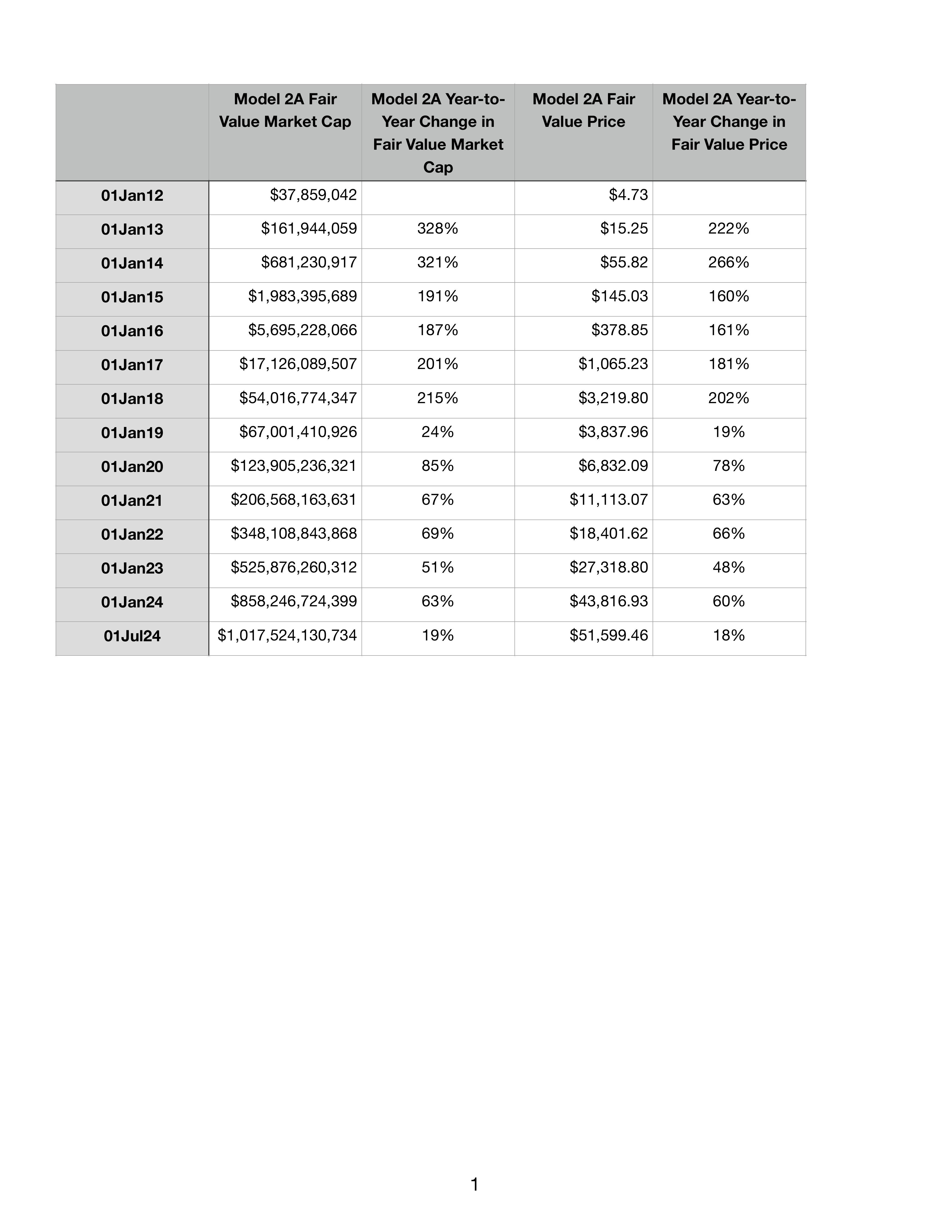
The Model 2A and 2B equations 11.5 and 11.6, respectively, can be used to compute the “Fair Value” Market Cap values for Bitcoin throughout its history. Since the Model 2A and 2B equations yield nearly identical results (Figures 11.7, 11.8 and 11.9), market cap and price were computed just from the Model 2A equation. These results are presented in Table 11.1.
The results of Table 11.1 illustrate the substantial reduction in the annual growth rate of market cap after 2018.
In addition, the ratio of observed Bitcoin market cap to the Model 2A equation for fair value market cap is presented in blue in Fig 11.10. The market cap rose to 23, 6.5, 2.5 and 4.8 times fair value in the “bull markets” (i.e., temporary price bubbles ) of 2013, 2017, 2019, and 2021. The magnitude of these temporary price bubbles has been declining, and this phenomenon seems likely to decline further in the future, as investors become more uniformly savvy about Bitcoin fair value.
The data points in red represent those days in which Bitcoin market cap was in the range of 1.5 times fair value down to 2/3 of fair value. This range, representing more than half of Bitcoin’s history, is viewed by the author as a “fair value range” — a range of typical Bitcoin market cap volatility in the periods between “bull markets”. According to Model 2A and 2B,

Fig 11.10 Ratio of Observed Bitcoin Market Cap to the Model 2A Fair Value Market Cap. The Bitcoin network has been prone to temporary price bubbles (2013, 2017, 2019, and 2021), when the growth Bitcoin market cap detaches temporarily detaches from the growth of network size. As computed using Model 2A (or Model 2B) the magnitude of the temporary price bubbles was 23-fold, 6.5-fold, 2.5-fold, and 4.8-fold in 2012, 2017, 2019 and 2021, respectively. The data points highlighted in red represent typical market cap and price volatility during the non-bubble periods — a range from 1.5 times fair value down to 2/3 of fair value.
Table 11.1 Bitcoin Fair Values for Market Cap and Price Computed from Model 2A Bitcoin “Fair Value” Market Cap and Prices are computed from Model 2A. (The results from Model 2B are nearly identical.) A decline in annual increases in market cap and price is evident after 2018.
11.8 Conclusions and Comments
Two new network value models were developed and applied to the Bitcoin network. Each of these two models was adaptable to either the SRET model format or the Power Law model format (with 2000 day offset).
Network Value Model 1
Model 1 has two equations, a first equation expressing network size, N, as a function of time, and a second equation expressing network value, V, as a function of time. As shown in Sections 11.2 and 11.3, these relationships define the relationship of V and N during each adoption period in which both V and N plot linearly. This relationship is of the form, V = c*Nx, where x and c are unique for each period.
From Model 1A (based on the SRET equation format), the relationships were
2012 to 2018: V = c*N1.97 , with c = 1.89 x 10⁴, and
2019 to 01Jul2024: V = c*N2.70 , with c = 1.08 x 10⁹
From Model 1B (based on the Power equation format, with 2000 day time offset), the relationships were comparable:
2012 to 2018: V = c*N1.96 , with c = 2.19 x 10⁴, and
2019 to 01Jul2024: V = c*N2.70 after 2018 with c = 1.12 x 10⁹.
These results reinforce the significance and magnitude of the 2018 change to the Bitcoin network. We had seen previously that the relationships of both V and N changed with regard to time, as shown in Figures 11.1 through 11.4. The new results above show that the relationships of V and N also changed to each other.
Network Value Model 2
Model 2 is a single equation relating the growth of network value, V, to the growth of network size and elapsed time. The most important outcome of this model is the linearity of the model throughout the period from 01Jan2012 to 01Jul2024 in spite of the substantial decline in Bitcoin network adoption rate starting in 2018.
Model 2 potentially provides an important new tool for understanding Bitcoin market cap fair value. For several years following the 2018 transition to a new adoption period, the SRET and Power Law models for fair value market cap for Period 2 were uncertain (Equations 11.2 and 11.4). The Period 1 equation was no longer accurate (as shown by the dashed line in Figures 11.2 and 11.4). Time was required for sufficient new data to emerge to define the slope and intercept of the Period 2 SRET and Power Law model equations.
During that transition period, the Model 2 plot of ln(V/N) retained its linearity in both the SRET model and Power Law model formats (Fig 11.5 and 11.6), providing an accurate calculation of the changing fair value market cap during the transition period.
Fourteen historic technology adoptions from the 20th and 21 centuries were reviewed in Substack Chapters 6 and 7. Most of these adoptions had a lifespan of 30 to 40 years, and most experienced 3 or 4 changes in adoption slope, like the change observed for Bitcoin in 2018. These historic adoption rate changes were sometimes decreases in adoption rate, and sometimes increases.
It has been six years since the 2018 change to the Bitcoin network. It is almost inevitable that another change in adoption rate will occur in the not too distant future — perhaps coinciding with the introduction of Bitcoin ETF’s in the US, and the wide scale acceptance of Bitcoin by many world governments. If the Model 2 plots of ln(V/N) in the SRET model and Power Law model formats continue to be linear (as in Figures 11.5 and 11.6), Model 2 could serve a useful role in navigating the transition period.
Network Value Models 1 and 2
Model 1 was expressed in terms of both the SRET model and the Power Law model (with 2000 day time offset). The results were very consistent between the two models.
Likewise, Model 2 results for the two different model equation formats were very consistent.
These results reinforce previous observations from Chapters 6 through 10 that the SRET model and the Power Law model (with 2000 day time offset) are both effective approaches for modeling technology adoptions.
11.9 References
Metcalfe, B. Metcalfe’s Law after 40 Years of Ethernet.Computer, 46(12): 26-31, 2013.
Alabi, K. Digital blockchain networks appear to be following Metcalfe’s Law. Electronic Commerce Research and Applications, 24: 23-29, 2017.
Peterson, TF. Metcalfe’s Law as a model for Bitcoin’s value, Alternative Investment Analyst Review, 7:9-18, 2018.
Van Vliet, B. An alternative model of Metcalfe’s Law for valuing Bitcoin. Economic Letters, 165: 70-72, 2018.
Alabi, KA. 2020 perspective on ‘Digital blockchain networks appear to be following Metcalfe’s Law’. Electronic Commerce Research and Applications, 40: 100939, 2020.
11.10 About the Author
The author has a B.S. and PhD. In chemical engineering. His PhD thesis focussed on mathematical modeling, simulation, and implementation of process control. Following his PhD, he was a university professor for 10 years at two US universities, focusing on both research and teaching. At both universities he taught the required chemical engineering course in process modeling and control. He subsequently spent more than 20 years in industrial chemical engineering practice.
11.11 Appendix 1: Mathematical Relationships and Solution Methodology
11.11.1 Deriving the Relationship Between V and N in Model 1A and Model 1B
The relationship of N to V from the two Model 1A equations is revealed by a simple derivation.
Assume that there is a relationship V = c*Nx. Then, this relationship becomes:
ln(V) = ln(c) + x*ln(N)
Setting this relationship for ln(V) equal to the Model 1A equation for ln(V), Eq 11.2
ln(c) + x*ln(N) = m2*sqrt(elapsed time) + b2
Which reduces to
ln(N) = (m2/x)*sqrt(elapsed time) + (b2-ln(c))/x
Examining this equation in comparison to Eq 11.1, ln(N) = m1*sqrt(elapsed time) + b1, the following relationships emerge
m1 = (m2/x), or x = m2/m1
and
b1 = (b2-ln(c))/x. which can be solved for c
ln(c) = b2 - x*b1
c = e(b2 - x*b1)
The same derivation applied to Model 1B (Equations 11.3 and 11.4, based on the Power Law equation format) leads to:
n1 = (n2/x), or x = n2/n1
and
d1 = (d2-ln(c))/x. which can be solved for c
ln(c) = d2 - x*d1
c = e(d2 - x*d1)
11.11.2 Methodology for Analysis of SRET Model and Power Law Model Plots
Most of the figures in this Substack Chapter involve plotting Bitcoin network data, then determining the slope and intercept of linear periods (e.g., Figures 11.1 through 11.6). The purpose of this section is to describe the common methodology employed for these analyses.
Bitcoin network data in this chapter are provided by the cryptocurrency analysis provider Glassnode (www.glassnode.com), as part of an “Advanced” membership plan, at about $30/month.
Day 1 of Bitcoin price and market cap history in the Glassnode database is 17Jul2010. The Glassnode daily market cap and Bitcoin-containing address counts are numbered from Day 1 through Day 5099 (01Jul2024). The period of primary focus in this Chapter is Day 534 (01Jan2012) to Day 5099 (01Jul2024).
The freezing of the data set at 01Jul2024 was based on the desire to have a consistent data set for the Substack analyses of Chapters 8, 9, 10 and 11. The intention of the author is to update the data set and analyses each successive January 1 and July 1.
Data analyses and preparation of figures were performed using Matlab (www.mathworks.com).
The plots of Model 1A and 1B equations for network size and network value (detailed in Chapters 8 and 9) resolved into two linear periods (Periods 1 and 2, before and after 2018). The slope and intercept of SRET model and Power Law model equations were determined separately for these two periods using the Matlab least-squares, best-fit algorithm .
The SRET and Power Law model plots for Model 2A and 2B were evaluated as a single linear period from 2012 to present (01Jul2024).
The first step in the determination of slope and intercept for a particular adoption period was choice of a criterion for data inclusion — that is, which days should be included from the 5099 days of Bitcoin history between 17Jul2010 to 01Jul2024. The overall goal of this criterion was to exclude data from Bitcoin history that reflects temporary Bitcoin price bubbles — periods when Bitcoin price temporarily detaches from network size — e.g., 2013, 2017, 2019, 2021.
Criterion for market cap analyses (Figures 11.2 and 11.4) and for analyses of Model 2 plots (Figures 11.5 and 11.6): days for inclusion must be less than 1.5 times the “fair value”, best-fitting, straight “blue” line through the included data, and greater than 2/3 of the fair-value line. This criteria excludes data points from the 2013, 2017, 2019 and 2021 “bull market” periods.
Criterion for analysis of Bitcoin-containing addresses (Figures 11.1 and 11.3): days for inclusion should be less than 1.05 times the “blue” fair value line and greater than 1/(1.05) times the fair value line. This criterion primarily excludes data points associated with temporary increases in address count associated with Bitcoin price bubbles.
Finally, the slope and intercept for a particular adoption period are determined by an iterative procedure:
Step 1: Make an initial guess at the slope and intercept —e.g., based on an algebraic calculation using two data points likely to be on or near the final best-fitting straight line.
Step 2: Determine the data points to be included in analyses based on this slope and intercept, using the inclusion criterion described above.
Step 3: Determine the slope and intercept of the best-fitting, least-squares, linear fit through these chosen data points.
Step 4: Repeat Steps 2 and 3 until the iterative process converges on a particular slope, intercept and set of data points. This convergence always happens, typically after 6 to 10 iterations — provided that the initial guess of slope and intercept are not too distant from the final values.
11.12 Appendix 2: Summary of Previous Substack Articles, with Links
Chapter 6. Modeling Technology Adoptions of the 20th and 21st Century: Part 1. When the Power Law Model Succeeds
Link:
https://bitcoinmodeler.substack.com/p/chapter-6-modeling-technology-adoptions?r=du1cn
Synopsis:
Analysis of 14 historic technology adoptions of the 20th and 21st century demonstrate that technology adoption is marked by rapid growth, but with a declining annual growth rate increase (Chapters 6 and 7). Furthermore, all 14 historic technology adoptions demonstrated that adoption does not occur in a smooth, consistent manner; rather, technology adoption occurs through a series of adoption periods, with distinct adoption rates — each with a higher or lower adoption rate than the previous period.
Seven historic technology adoptions are examined in Chapter 6, by two models:
Power Law Model: ln(N) = n*ln(elapsed time + time offset) + d
Square Root of Elapsed Time (SRET): ln(N) = m*sqrt(elapsed time) + b
Where n, m, d and b are constants determined as the slopes and intercepts of each linear period. The time offset was 0 for the analyses in Chapter 6.
For these seven historic technology adoptions, both the Power Law model with 0 time offset and the SRET model are effective in linearizing the adoption data — that is, manipulating the position of individual adoption data points to convert the curved shape of the semilog graph of adoption versus time to a sequence of straight lines representing the individual adoption periods.
To be clear: The Power Law model with 0 time offset and the SRET model do not lead to identical plots for these seven historic technology adoptions. The Power Law model with 0 time offset is much more intense in its manipulation of adoption data. But, the SRET model and the Power Law model identify the same historical adoption periods in each of the seven examples.
For the seven historic technology adoptions of Chapter 6, both the SRET model and the Power Law model demonstrate that a typical technology adoption is marked by multiple different linear periods over its history.
Chapter 7. Modeling Technology Adoptions of the 20th and 21st Century: Part 2. When the Power Law Model Fails
link:
https://bitcoinmodeler.substack.com/p/chapter-7-modeling-technology-adoptions?r=du1cn
Synopsis:
Seven additional historic technology adoptions of the 20th and 21st century were examined. The SRET model was effective in linearizing the adoption data for all seven cases.
The Power Law model with 0 time offset, ln(N) = n*ln(elapsed time) + d, WAS NOT effective in linearizing these seven historic adoptions — the movement of data points by the Power Law model (with no time offset) was too intense, resulting in clear evidence of data distortion. The Power Law modeling approach was effective after inclusion of a non-zero value of the time offset. This time offset has the effect of reducing the intensity of the Power Law model — i.e., higher time offset value —> lower Power Law intensity.
Power Law ln(N) = n*ln(elapsed time + time offset) + d
Square Root of Elapsed Time (SRET): ln(N) = m*sqrt(elapsed time) + b
Where n, m, d and b are constants determined as the slopes and intercepts of each linear period. The time offset is a constant chosen to appropriately linearize the adoption data.
The values of time offset to appropriately linearize the seven historic adoptions of Chapter 7 were: 4 years (Fig 7.6), 5 years (Fig 7.11), 3 years (Fig 7.24), 2 years (Fig 7.34), 6 years (Fig 7.44), 3 years (Fig 7.54), and 4 years (Fig 7.64).
With an optimum time offset of 5 years, the second historic technology adoption above revealed 4 linear adoption periods over its 28-year history, matching the results from the SRET model for the same historic adoption (Fig 7.7). However, when a suboptimal time offset of 1 year was evaluated for this technology adoption, the data point locations were distorted to appear that there was just one single, long adoption period (Fig 7.12). This result raises a serious note of caution about the application of the Power Law model with time offset. A suboptimal value of the time offset can sometimes lead to very misleading results.
This result is significant because a similar case arises in Substack Chapter 9, the application of the Power Law to modeling Bitcoin market cap.
Chapter 8. Application of the Power Law and SRET Models to the Growth of Bitcoin Market Size
link:
https://bitcoinmodeler.substack.com/p/chapter-8-analyzing-the-growth-of?r=du1cn
The count of Bitcoin-containing addresses is shown to be a reasonable metric for modeling Bitcoin network size. The SRET model effectively models the growth of Bitcoin network size. Of particular interest is a sharp decline in the Bitcoin-containing address growth trajectory in 2018, dividing Bitcoin’s history into two distinct linear periods — 2012 to 2018 (Period 1), and 2019 to present (Period 2).
This 2018 decline in the adoption rate of network size is confirmed by an independent set of adoption data from Glassnode and Willy Woo.
The Power Law Model with a 2000 day time offset (5.5 years) is demonstrated to be a reasonable choice to: 1) attain alignment between Period 1 and 2 data, and 2) match the SRET model results.
Note: It is not necessary for Bitcoin-containing address count or any other metric to be an exact measure of Bitcoin network size. To be effective in the modeling presented in these Substack chapters, the chosen metric must just retain the same proportionality to network size.
Chapter 9. Application of the Power Law and SRET Models to the Growth of Bitcoin Market Cap
link:
https://bitcoinmodeler.substack.com/p/chapter-9-application-of-the-power?r=du1cn
Market Capitalization is the metric for modeling Bitcoin network value. The SRET model effectively models the growth of Bitcoin network value. Mirroring the result obtained in Chapter 8 for network size, a sharp decline in the market cap growth trajectory is observed at the end of 2018, dividing Bitcoin’s history into two distinct linear periods — 2012 to 2018 (Period 1), and 2019 to present (Period 2).
The Power Law Model with a 2000 day time offset (5.5 years) is demonstrated to be a reasonable choice to: 1) attain alignment of data between Periods 1 and 2, and 2) to match the SRET model results.
A disturbing result presented in this Chapter is the observation that a suboptimal time offset of 560 days (~1.5 years) results in the appearance of data linearity from 2012 to present — the appearance that there was no change in market cap trajectory before or after 2018. This result parallels the aberrant result observed in Chapter 7 for the Power Law model with a suboptimal time offset.
The time offset of 560 days is the value chosen by Giovanni Santostasi for the popular, Twitter version of the Power Law model applied to Bitcoin market cap. A feature of this model is the claim that Bitcoin has been on a single, linear trajectory throughout its history. The analyses of Chapters 7 through 9 conclude that this apparent linearity of the Santostasi model is just the misleading result of a suboptimal choice of a 560-day time offset .
Chapter 10. Visualizing Power Law Success and Failure
link:
https://bitcoinmodeler.substack.com/p/chapter-10-visualizing-power-law?r=du1cn
Semilog plots of technology adoption as a function of time were presented for 14 different technology adoptions of the 20th and 21st centuries in Chapters 6 and 7. Comparable plots of Bitcoin-containing addresses and Bitcoin market cap were presented in Chapters 8 and 9.
These 16 semilog plots versus time share the same basic shape. They are concave-shaped — continuously rising, but with a gradually declining rate of annual increase.
The desired effect of the SRET and Power Law models is to translate the concave shape of the semilog plot described above into a linear plot in the SRET model or Power Law formats.
The purpose of Chapter 10 is to understand the efficacy of the SRET and Power Law model approaches by following the movements of individual adoption data points as they move from their original positions on the concave, semilog plot vs time to their final positions on a SRET model or Power Law model plot.
The “relatively gentle” SRET model was effective in each of the 16 cases above in converting the concave semilog plot into a linear plot suitable for modeling.
The plots in Chapter 10 (and Chapter 7) show how the Power Law model with 0 time offset often moves individual points much too aggressively, translating the concave shape of the semilog plot vs time into an aberrant, distorted convex shape. Addition of a Power Law non-zero time offset moves the individual data points back toward the desired linear alignment. For Bitcoin, the time offset of 560 days (the Santostasi value) brings the data points halfway back toward appropriate alignment. The time offset of 2000 days brings the data points into appropriate, linear alignment, The shape of the Power Law plot with 2000 day offset is identical to the SRET model plot of the same data.